The hardware and bandwidth for this mirror is donated by METANET, the Webhosting and Full Service-Cloud Provider.
If you wish to report a bug, or if you are interested in having us mirror your free-software or open-source project, please feel free to contact us at mirror[@]metanet.ch.
This package is intended to help data scientists and decision-makers understand the potential value of churn prediction models depending on how many customers are being targeted by a campaign.
You can install the development version from GitHub with:
# install.packages("devtools")
devtools::install_github("PeerChristensen/modelimpact")The first three functions aim to provide information about the
business impact of using a model and targeting x % of the customer base.
These functions accept the following arguments (required ones in
bold):
x - a data frame fixed_cost - fixed costs (defaults to 0) var_cost - variable costs (defaults to 0) tp_val - true positive value (defaults to 0) prob_col - the variable containing
target class probabilitiestruth_col the variable containing the
actual classprofit_thresholds() accepts the following arguments:
x - a data frame var_cost - variable costs prob_accept - Probability of offer being accepted.
Defaults to 1. tp_val - The average value of a True Positive.
var_cost is automatically subtracted. fp_val - The average cost of a False Positive.
var_cost is automatically subtracted. tn_val - The average cost of a True Negatives fn_val - The average cost of a False Negatives
prob_col - The column with
probabilities of the event of interest truth_col - the column with the actual
outcome/class. Possible values are ‘Yes’ and ‘No’# Parameter settings
fixed_cost <- 1000
var_cost <- 100
tp_val <- 2000library(modelimpact)
library(tidyverse)
library(scales)
head(predictions)
#> # A tibble: 6 x 4
#> predict No Yes Churn
#> <chr> <dbl> <dbl> <chr>
#> 1 No 0.996 0.00353 No
#> 2 No 0.983 0.0166 No
#> 3 No 0.993 0.00705 No
#> 4 No 0.981 0.0187 No
#> 5 No 0.894 0.106 No
#> 6 No 0.997 0.00254 Nocost_rev <- predictions %>%
cost_revenue(
fixed_cost = fixed_cost,
var_cost = var_cost,
tp_val = tp_val,
prob_col = Yes,
truth_col = Churn)
head(cost_rev)
#> # A tibble: 6 x 4
#> row pct cost_sum cum_rev
#> <int> <int> <dbl> <dbl>
#> 1 1 1 1100 2000
#> 2 2 1 1200 4000
#> 3 3 1 1300 6000
#> 4 4 1 1400 6000
#> 5 5 1 1500 6000
#> 6 6 1 1600 8000# functions for formatting plotting axes
ks <- function (x) { number_format(accuracy = 1,
scale = 1/1000,
suffix = "k",
big.mark = ",")(x) }
pcts <- function (x) { percent_format(scale=1)((x / max(x)) * 100) }
theme_set(theme_minimal())
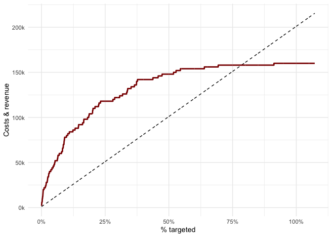
cost_rev %>%
ggplot() +
geom_line(aes(row,cost_sum), colour ="black",linetype="dashed") +
geom_line(aes(row,cum_rev), colour = "darkred",size=1) +
scale_y_continuous(labels = ks) +
scale_x_continuous(labels = pcts) +
labs(x = "% targeted",y = "Costs & revenue")
profit_df <- predictions %>%
  profit(
    fixed_cost = fixed_cost,
    var_cost   = var_cost,
    tp_val     = tp_val,
    prob_col   = Yes,
    truth_col  = Churn)

head(profit_df)
#> # A tibble: 6 x 3
#>     row   pct profit
#>   <int> <int>  <dbl>
#> 1     1     1    900
#> 2     2     1   2800
#> 3     3     1   4700
#> 4     4     1   4600
#> 5     5     1   4500
#> 6     6     1   6400
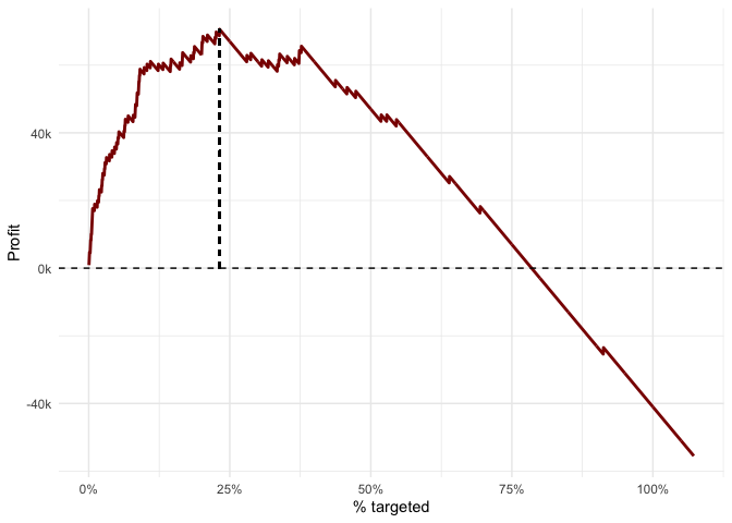
# max profit
max_profit <- profit_df %>% filter(profit == max(profit)) %>% select(row,pct,profit)
max_profit
#> # A tibble: 1 x 3
#> row pct profit
#> <int> <int> <dbl>
#> 1 464 22 70600profit_df %>%
ggplot(aes(x=row,y=profit)) +
geom_line(colour = "darkred",size=1) +
scale_y_continuous(labels = ks) +
geom_segment(x = max_profit$row, y= 0,xend=max_profit$row,
yend = max_profit$profit, colour="black",linetype="dashed") +
geom_hline(yintercept = 0,colour="black", linetype="dashed") +
scale_x_continuous(labels = pcts) +
labs(x = "% targeted",y = "Profit")
roi_df <- predictions %>%
  roi(
    fixed_cost = fixed_cost,
    var_cost   = var_cost,
    tp_val     = tp_val,
    prob_col   = Yes,
    truth_col  = Churn)

head(roi_df)
#> # A tibble: 6 x 5
#>     row   pct cum_rev cost_sum   roi
#>   <int> <int>   <dbl>    <dbl> <dbl>
#> 1     1     1    2000     1100 0.818
#> 2     2     1    4000     1200 2.33
#> 3     3     1    6000     1300 3.62
#> 4     4     1    6000     1400 3.29
#> 5     5     1    6000     1500 3
#> 6     6     1    8000     1600 4
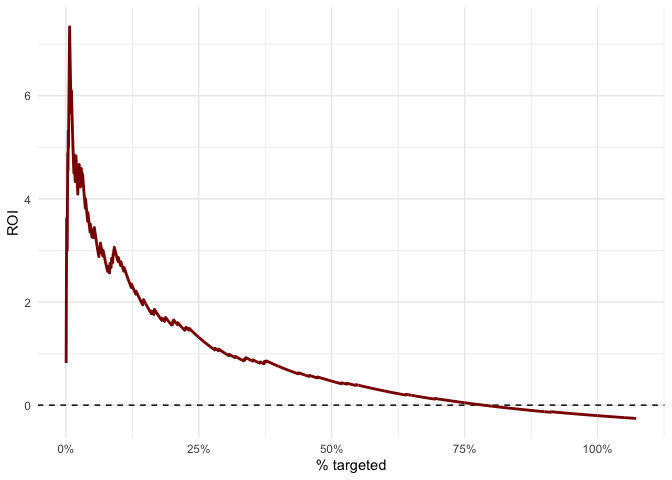
roi_df %>%
ggplot(aes(x=row,y=roi)) +
geom_hline(yintercept = 0,colour="black", linetype="dashed") +
geom_line(colour = "darkred",size=1) +
scale_x_continuous(labels = pcts) +
labs(x = "% targeted",y = "ROI")
thresholds <- predictions %>%
  profit_thresholds(var_cost    = 100,
                    prob_accept = .7,
                    tp_val      = 2000,
                    fp_val      = 0,
                    tn_val      = 0,
                    fn_val      = -2000,
                    prob_col = Yes,
                    truth_col = Churn)

head(thresholds)
#> # A tibble: 6 x 2
#>   threshold payoff
#>       <dbl>  <dbl>
#> 1      0      9850
#> 2      0.01  68400
#> 3      0.02  67500
#> 4      0.03  42700
#> 5      0.04  42960
#> 6      0.05  20840
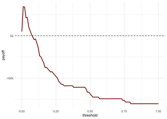
optimal_threshold <- thresholds %>% filter(payoff == max(payoff))
optimal_threshold
#> # A tibble: 1 x 2
#> threshold payoff
#> <dbl> <dbl>
#> 1 0.01 68400thresholds %>%
ggplot(aes(x=threshold,y=payoff)) +
geom_line(color="darkred",size = 1) +
geom_hline(yintercept=0,linetype="dashed") +
scale_y_continuous(labels = ks)
These binaries (installable software) and packages are in development.
They may not be fully stable and should be used with caution. We make no claims about them.