

The hardware and bandwidth for this mirror is donated by METANET, the Webhosting and Full Service-Cloud Provider.
If you wish to report a bug, or if you are interested in having us mirror your free-software or open-source project, please feel free to contact us at mirror[@]metanet.ch.
neuralsbi is an R-native package for Neural Simulation-based
inference.
Neural estimators are implemented directly in R on the torch R package.
# install.packages("remotes")
remotes::install_github("pedroliman/neuralsbi")

# the neural back end (once)
install.packages("torch")
torch::install_torch()Simulation-based inference fits a posterior from a prior and a
simulator, with no likelihood required. To keep the setup familiar, here
is ordinary linear regression written as a simulator: a response
y scattered around a line,
y ~ Normal(alpha + beta * x, sigma) — the same model you
might write in Stan. Its likelihood is easy to write down, which is
exactly what makes it a good check: we know the coefficients that
generated the data, so we can confirm the posterior recovers them.
library(neuralsbi)
set.seed(1)

# Regression design: a single covariate x, measured at 50 fixed points.
N <- 50
x <- seq(-1, 1, length.out = N)

# Simulator: given rows of (alpha, beta, sigma), draw one response vector y each
# from y ~ Normal(alpha + beta * x, sigma). Fully vectorised over the rows of
# theta, and it only generates data — no fitting happens here.
simulator <- function(theta) {
  alpha <- theta[, 1]
  beta  <- theta[, 2]
  sigma <- theta[, 3]
  mu <- outer(beta, x) + alpha                       # row i is the line alpha_i + beta_i * x
  mu + matrix(rnorm(length(mu)), nrow(mu)) * sigma   # add row-specific Gaussian noise
}

# Priors over the intercept, slope, and noise scale, then train the posterior.
prior <- prior_uniform(low = c(-3, -3, 0.1), high = c(3, 3, 2))
fit   <- npe(prior, simulator, n_simulations = 10000, seed = 1)

# Simulate one data set from known coefficients, then infer them back. The
# observation the posterior conditions on is the response vector y.
theta_true <- c(alpha = 2, beta = -1, sigma = 0.5)
set.seed(38)                       # a fixed, representative data set
y_obs      <- simulator(rbind(theta_true))
post       <- posterior(fit, x_obs = y_obs)
draws      <- sample(post, 10000)
The posterior mean recovers the coefficients that generated the data:
rbind(truth = theta_true, posterior_mean = colMeans(draws))
#>                   alpha      beta     sigma
#> truth          2.000000 -1.000000 0.5000000
#> posterior_mean 2.003668 -1.041009 0.5003288pairplot(draws, truth = theta_true, labels = c("alpha", "beta", "sigma"))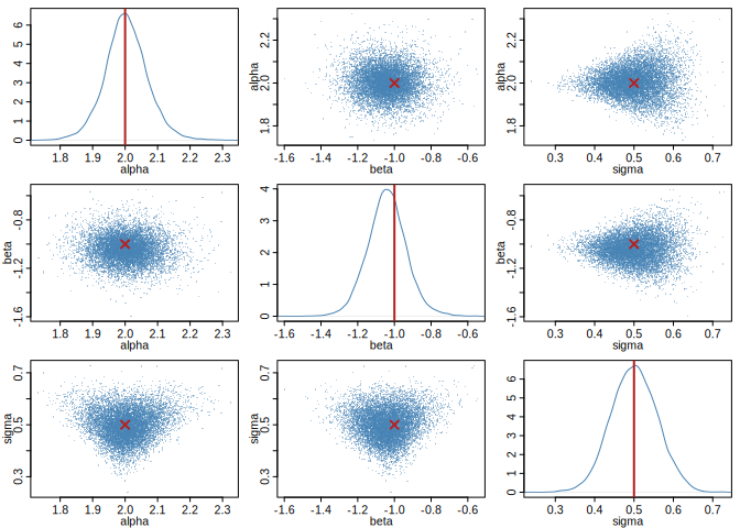
The same posterior gives a point estimate; calibration checks such as
simulation-based calibration live in
vignette("diagnostics").
map_estimate(post)     # posterior mode
#> [1]  1.9989619 -1.0442036  0.4702335
If you’re interested in sbi in other languages or functionality not available here, see the awesome neural SBI repo; there are some good implementations in python and in Julia.
The package website has four vignettes that build on each other:
MIT
These binaries (installable software) and packages are in development.
They may not be fully stable and should be used with caution. We make no claims about them.