The hardware and bandwidth for this mirror is donated by METANET, the Webhosting and Full Service-Cloud Provider.
If you wish to report a bug, or if you are interested in having us mirror your free-software or open-source project, please feel free to contact us at mirror[@]metanet.ch.
partition is a fast and flexible framework for agglomerative partitioning. partition uses an approach called Direct-Measure-Reduce to create new variables that maintain the user-specified minimum level of information. Each reduced variable is also interpretable: the original variables map to one and only one variable in the reduced data set. partition is flexible, as well: how variables are selected to reduce, how information loss is measured, and the way data is reduced can all be customized.
You can install the partition from CRAN with:
install.packages("partition")Or you can install the development version of partition GitHub with:
# install.packages("remotes")
remotes::install_github("USCbiostats/partition")library(partition)
set.seed(1234)
df <- simulate_block_data(c(3, 4, 5), lower_corr = .4, upper_corr = .6, n = 100)
# don't accept reductions where information < .6
prt <- partition(df, threshold = .6)
prt
#> Partitioner:
#> Director: Minimum Distance (Pearson)
#> Metric: Intraclass Correlation
#> Reducer: Scaled Mean
#>
#> Reduced Variables:
#> 1 reduced variables created from 2 observed variables
#>
#> Mappings:
#> reduced_var_1 = {block2_x3, block2_x4}
#>
#> Minimum information:
#> 0.602
# return reduced data
partition_scores(prt)
#> # A tibble: 100 × 11
#> block1_x1 block1_x2 block1_x3 block2_x1 block2_x2 block3_x1 block3_x2
#> <dbl> <dbl> <dbl> <dbl> <dbl> <dbl> <dbl>
#> 1 -1.00 -0.344 1.35 -0.526 -1.25 1.13 0.357
#> 2 0.518 -0.434 -0.361 -1.48 -1.53 -0.317 0.290
#> 3 -1.77 -0.913 -0.722 0.122 0.224 -0.529 0.114
#> 4 -1.49 -0.998 0.189 0.149 -0.994 -0.433 0.0120
#> 5 0.616 0.0211 0.895 1.09 -1.25 0.440 -0.550
#> 6 0.0765 0.522 1.20 -0.152 -0.419 -0.912 -0.362
#> 7 1.74 0.0993 -0.654 -1.26 -0.502 -0.792 -1.03
#> 8 1.05 2.19 0.913 0.254 0.328 -1.07 -0.976
#> 9 -1.07 -0.292 -0.763 0.437 0.739 0.899 -0.342
#> 10 -1.02 -0.959 -1.33 -1.57 -1.11 0.618 0.153
#> # ℹ 90 more rows
#> # ℹ 4 more variables: block3_x3 <dbl>, block3_x4 <dbl>, block3_x5 <dbl>,
#> # reduced_var_1 <dbl>
# access mapping keys
mapping_key(prt)
#> # A tibble: 11 × 4
#> variable mapping information indices
#> <chr> <list> <dbl> <list>
#> 1 block1_x1 <chr [1]> 1 <int [1]>
#> 2 block1_x2 <chr [1]> 1 <int [1]>
#> 3 block1_x3 <chr [1]> 1 <int [1]>
#> 4 block2_x1 <chr [1]> 1 <int [1]>
#> 5 block2_x2 <chr [1]> 1 <int [1]>
#> 6 block3_x1 <chr [1]> 1 <int [1]>
#> 7 block3_x2 <chr [1]> 1 <int [1]>
#> 8 block3_x3 <chr [1]> 1 <int [1]>
#> 9 block3_x4 <chr [1]> 1 <int [1]>
#> 10 block3_x5 <chr [1]> 1 <int [1]>
#> 11 reduced_var_1 <chr [2]> 0.602 <int [2]>
unnest_mappings(prt)
#> # A tibble: 12 × 4
#> variable mapping information indices
#> <chr> <chr> <dbl> <int>
#> 1 block1_x1 block1_x1 1 1
#> 2 block1_x2 block1_x2 1 2
#> 3 block1_x3 block1_x3 1 3
#> 4 block2_x1 block2_x1 1 4
#> 5 block2_x2 block2_x2 1 5
#> 6 block3_x1 block3_x1 1 8
#> 7 block3_x2 block3_x2 1 9
#> 8 block3_x3 block3_x3 1 10
#> 9 block3_x4 block3_x4 1 11
#> 10 block3_x5 block3_x5 1 12
#> 11 reduced_var_1 block2_x3 0.602 6
#> 12 reduced_var_1 block2_x4 0.602 7
# use a lower threshold of information loss
partition(df, threshold = .5, partitioner = part_kmeans())
#> Partitioner:
#> Director: <custom director>
#> Metric: <custom metric>
#> Reducer: <custom reducer>
#>
#> Reduced Variables:
#> 2 reduced variables created from 7 observed variables
#>
#> Mappings:
#> reduced_var_1 = {block3_x1, block3_x2, block3_x5}
#> reduced_var_2 = {block2_x1, block2_x2, block2_x3, block2_x4}
#>
#> Minimum information:
#> 0.508
# use a custom partitioner
part_icc_rowmeans <- replace_partitioner(
part_icc,
reduce = as_reducer(rowMeans)
)
partition(df, threshold = .6, partitioner = part_icc_rowmeans)
#> Partitioner:
#> Director: Minimum Distance (Pearson)
#> Metric: Intraclass Correlation
#> Reducer: <custom reducer>
#>
#> Reduced Variables:
#> 1 reduced variables created from 2 observed variables
#>
#> Mappings:
#> reduced_var_1 = {block2_x3, block2_x4}
#>
#> Minimum information:
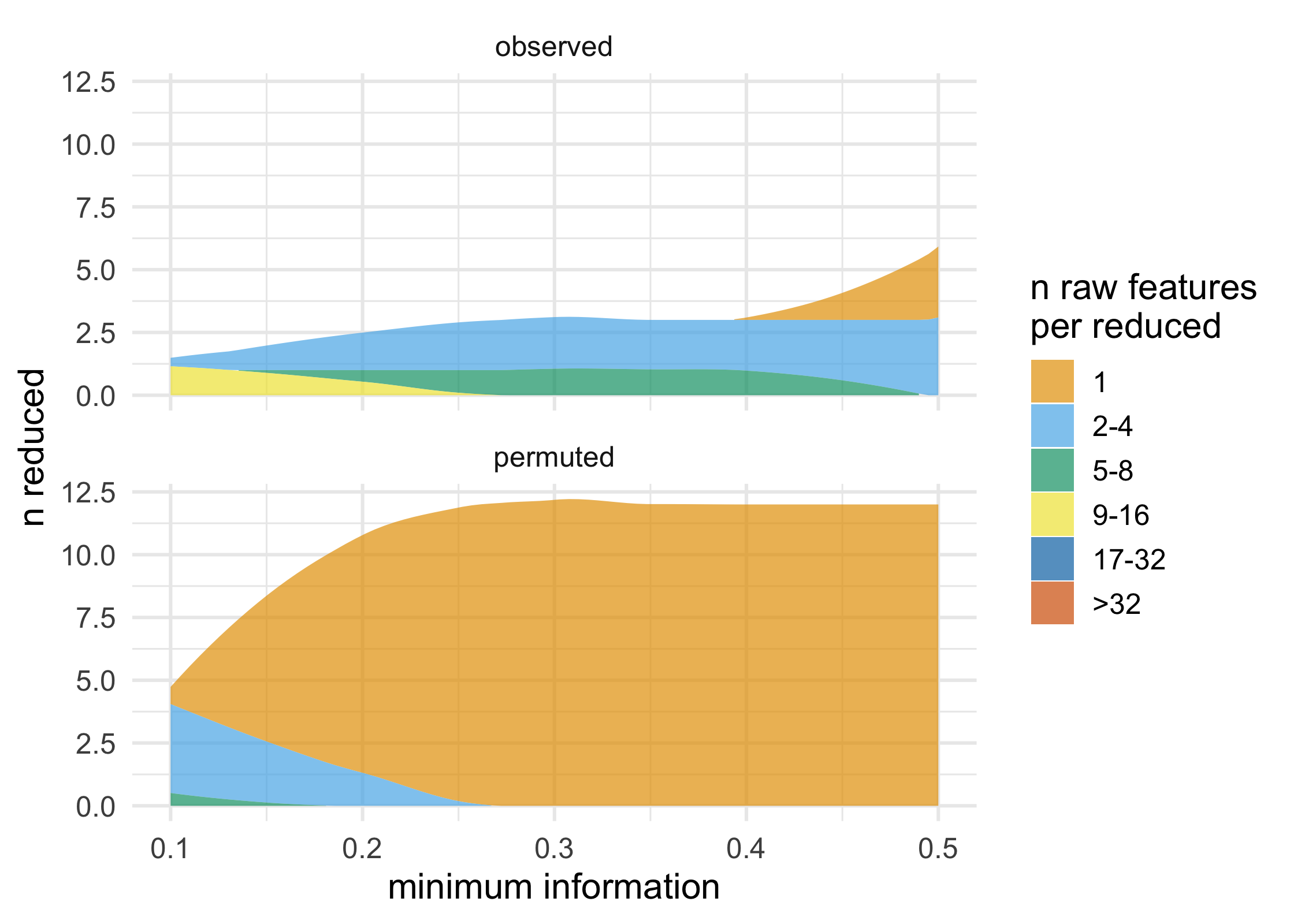
#> 0.602partition also supports a number of ways to visualize partitions and
permutation tests; these functions all start with plot_*().
These functions all return ggplots and can thus be extended using
ggplot2.
plot_stacked_area_clusters(df) +
  ggplot2::theme_minimal(14)
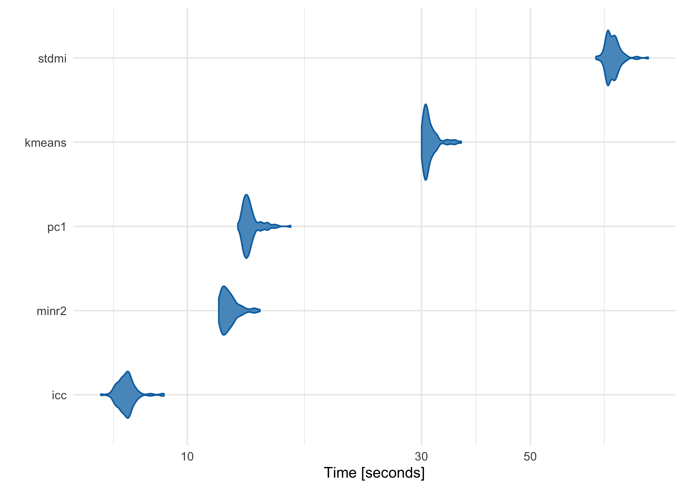
partition has been meticulously benchmarked and profiled to improve performance, and key sections are written in C++ or use C++-based packages. Using a data frame with 1 million rows on a 2017 MacBook Pro with 16 GB RAM, here’s how each of the built-in partitioners perform:
large_df <- simulate_block_data(c(3, 4, 5), lower_corr = .4, upper_corr = .6, n = 1e6)

basic_benchmarks <- microbenchmark::microbenchmark(
  icc = partition(large_df, .3),
  kmeans = partition(large_df, .3, partitioner = part_kmeans()),
  minr2 = partition(large_df, .3, partitioner = part_minr2()),
  pc1 = partition(large_df, .3, partitioner = part_pc1()),
  stdmi = partition(large_df, .3, partitioner = part_stdmi())
)
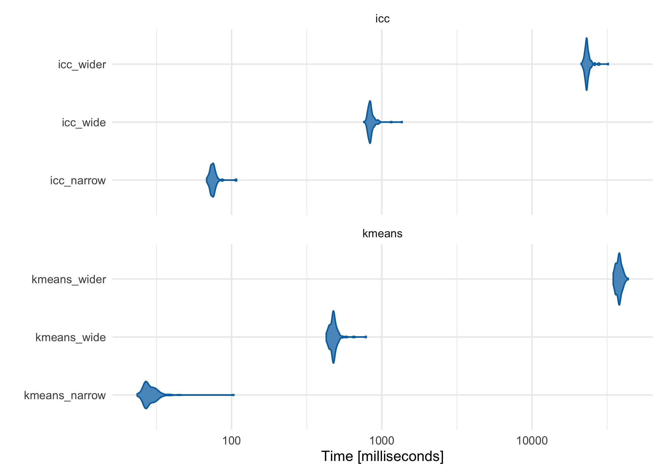
As the features (columns) in the data set become greater than the number of observations (rows), the default ICC method scales more linearly than K-Means-based methods. While K-Means is often faster at lower dimensions, it becomes slower as the features outnumber the observations. For example, using three data sets with increasing numbers of columns, K-Means starts as the fastest and gets increasingly slower, although in this case it is still comparable to ICC:
narrow_df <- simulate_block_data(3:5, lower_corr = .4, upper_corr = .6, n = 100)
wide_df <- simulate_block_data(rep(3:10, 2), lower_corr = .4, upper_corr = .6, n = 100)
wider_df <- simulate_block_data(rep(3:20, 4), lower_corr = .4, upper_corr = .6, n = 100)

icc_kmeans_benchmarks <- microbenchmark::microbenchmark(
  icc_narrow = partition(narrow_df, .3),
  icc_wide = partition(wide_df, .3),
  icc_wider = partition(wider_df, .3),
  kmeans_narrow = partition(narrow_df, .3, partitioner = part_kmeans()),
  kmeans_wide = partition(wide_df, .3, partitioner = part_kmeans()),
  kmeans_wider  = partition(wider_df, .3, partitioner = part_kmeans())
)
For more information, see our paper in Bioinformatics, which discusses these issues in more depth (Millstein et al. 2020).
Please read the Contributor Guidelines prior to submitting a pull request to partition. Also note that this project is released with a Contributor Code of Conduct. By participating in this project you agree to abide by its terms.
These binaries (installable software) and packages are in development.
They may not be fully stable and should be used with caution. We make no claims about them.