The hardware and bandwidth for this mirror is donated by METANET, the Webhosting and Full Service-Cloud Provider.
If you wish to report a bug, or if you are interested in having us mirror your free-software or open-source project, please feel free to contact us at mirror[@]metanet.ch.

plotor

The goal of plotor is to generate Odds Ratio plots from logistic regression models.

Installation

You can install the development version of plotor from GitHub with:

# install.packages("devtools")
devtools::install_github("craig-parylo/plotor")

You can also install the latest released version from Cran with:

install.packages("plotor")

Example

In this example we will explore the likelihood of surviving the Titanic disaster based on passenger economic status (class), sex, and age group.

In addition to plotor the packages we will use include dplyr, tidyr and forcats for general data wrangling, the stats package to conduct the logistic regression followed by broom to tidy the output and convert the results to Odds Ratios and confidence intervals, then ggplot2 to visualise the plot.

library(plotor)      # generates Odds Ratio plots
library(datasets)    # source of example data
library(dplyr)       # data wrangling
library(tidyr)       # data wrangling - uncounting aggregated data
library(forcats)     # data wrangling - handling factor variables
library(stats)       # perform logistic regression using glm function
library(broom)       # tidying glm model and producing OR and CI
library(ggplot2)     # data visualisation

Start with getting the data from the datasets package.

df <- datasets::Titanic |> 
  as_tibble() |> 
  # convert counts to observations
  filter(n > 0) |>
  uncount(weights = n) |>
  # convert categorical variables to factors.
  # we specify an order for levels in Class and Survival, otherwise ordering
  # in descending order of frequency
  mutate(
    Class = Class |>
      fct(levels = c('1st', '2nd', '3rd', 'Crew')),
    Sex = Sex |>
      fct_infreq(),
    Age = Age |>
      fct_infreq(),
    Survived = Survived |>
      fct(levels = c('No', 'Yes'))
  )

We now have a tibble of data containing four columns:

• Survived - our outcome variable describing whether the passenger survived Yes or died No,

• Class - the passenger class, either 1st, 2nd, 3rd or Crew,

• Sex - the gender of the passenger, either Male or Female,

• Age - whether the passenger was an Adult or Child.

We next conduct a logistic regression of survival (as a binary factor: ‘yes’ and ‘no’) against the characteristics of passenger class, sex and age group. For this we use the Generalised Linear Model function (glm) from the stats package, specifying:

• the family as ‘binomial’, and

• the formula as survival being a function of Class, Sex and Age.

# conduct a logistic regression of survival against the other variables
lr <- glm(
  data = df, 
  family = 'binomial', 
  formula = Survived ~ Class + Sex + Age
  )

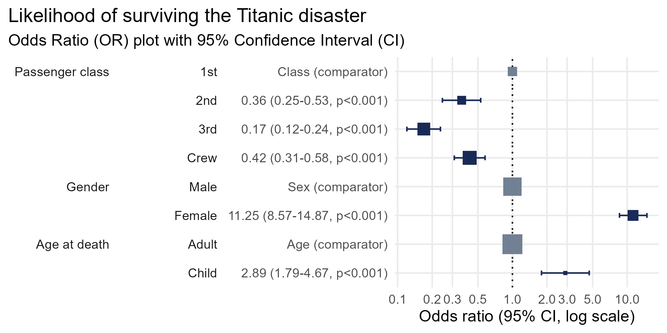
Finally, we can plot the Odds Ratio of survival using the plot_or function.

# using plot_or 
plot_or(glm_model_results = lr)

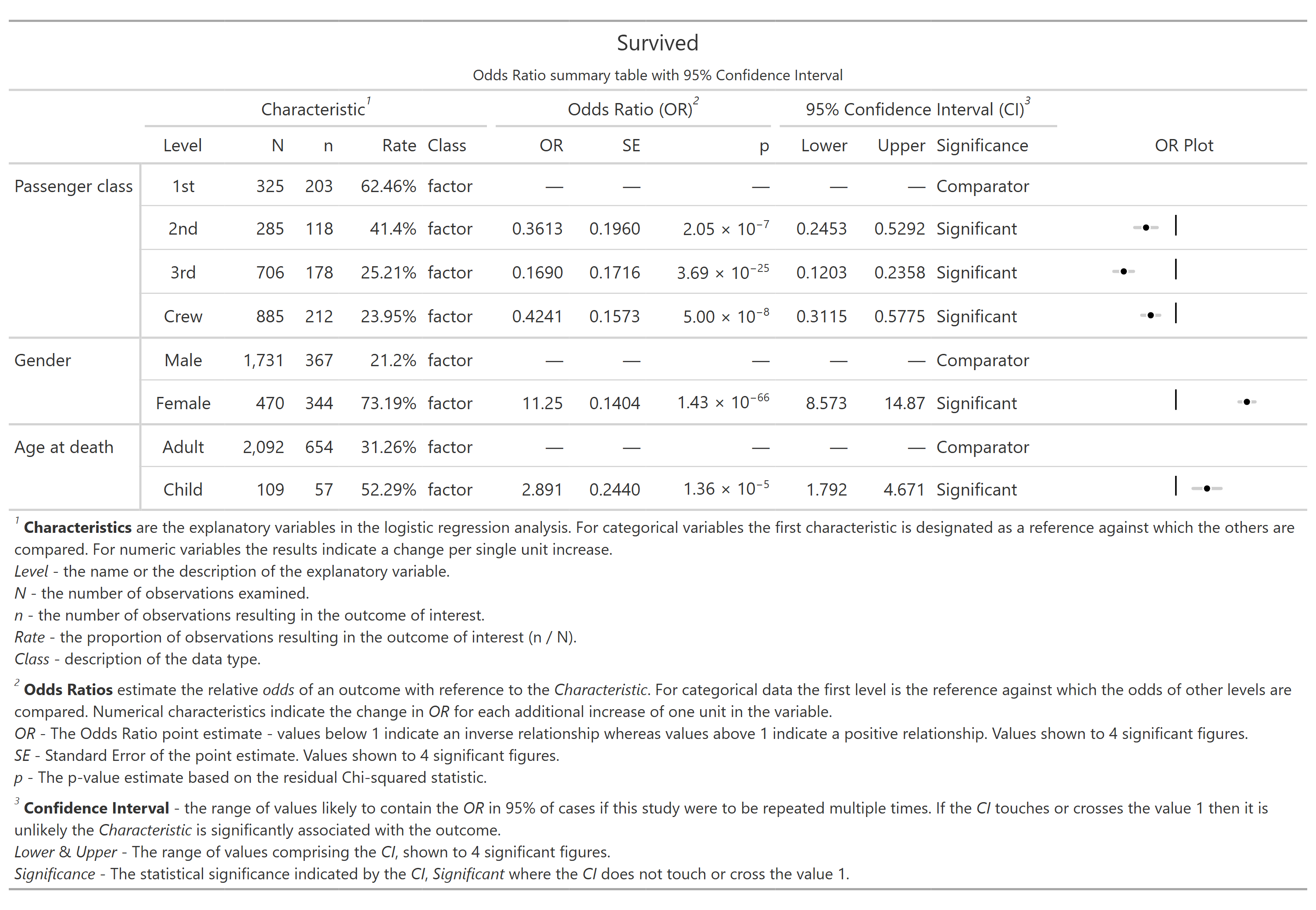
This plot makes it clear that:

• Children were 2.89 times more likely to survive than Adults,

• Passengers in 2nd, 3rd class as well as Crew were all less likely to survive than those in 1st class,

• Women were 11.25 times more likely to survive than men.

These binaries (installable software) and packages are in development.
They may not be fully stable and should be used with caution. We make no claims about them.