The hardware and bandwidth for this mirror is donated by METANET, the Webhosting and Full Service-Cloud Provider.
If you wish to report a bug, or if you are interested in having us mirror your free-software or open-source project, please feel free to contact us at mirror[@]metanet.ch.

R package to simulate Probabilistic Long-Term Effects in models with temporal dependence

Christopher Gandrud and Laron K. Williams

Version: 1.0

About

pltesim implements Williams’s (2016) method for simulating probabilistic long-term effects in models with temporal dependence.

It is built on the coreSim package.

Process

To find and show probabilistic long-term effects in models with temporal dependence with pltesim:

1. Estimate the coefficients. Currently pltesim works with binary outcome models, e.g. logit, so use glm from the default R installation.

2. Create a data frame with your counterfactual. This should have a row with the fitted counterfactual values and columns with names matching those in your fitted model. All variables without values will be treated as 0 in the counterfactual.

3. Simulate the long-term effects with plte_builder.

4. Plot the results with plte_plot.

Examples

These examples replicate Figure 1 in Williams (2016). First estimate your model. You may need to use btscs to generate spells for the binary dependent variable.

library(pltesim)
library(ggplot2)

data('negative_year')

# BTSCS set the data
neg_set <- btscs(df = negative_year, event = 'y', t_var = 'year',
                 cs_unit = 'group', pad_ts = FALSE)

# Estimate the model
m1 <- glm(y ~ x + spell_time + I(spell_time^2) + I(spell_time^3),
          family = binomial(link = 'logit'),
          data = neg_set)

Then fit the counterfactual:

counterfactual <- data.frame(x = 0.5)

Now simulate and plot long-term effects for a variety of scenarios using plte_builder and plte_plot. plte_builder takes as its input the fitted model object with the estimated coefficients (obj), an identification of the basic time period variable (obj_tvar), the counterfactual (cf), how long the counterfactual persists (cf_duration, it is permanent by default), and the time period points over which to simulate the effects.

Note that by default the predicted probabilities from logistic regression models are found. You can specify a custom quantity of interest function with the FUN argument.

In this first example the counterfactual is persistent throughout the entire time span:

# Permanent
sim1 <- plte_builder(obj = m1, obj_tvar = 'spell_time',
                     cf = counterfactual, t_points = c(13, 25))

plte_plot(sim1) + ggtitle('Permanent')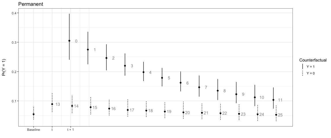

Note that the numbers next to each simulation point indicate the time since the last event. You can choose to not show these numbers by setting t_labels = FALSE in the plte_plot call.

In the next example, the effect only lasts for one time period:

# One-time
sim2 <- plte_builder(obj = m1, obj_tvar = 'spell_time', cf_duration = 'one-time',
                     cf = counterfactual, t_points = c(13, 25))

plte_plot(sim2) + ggtitle('One-time')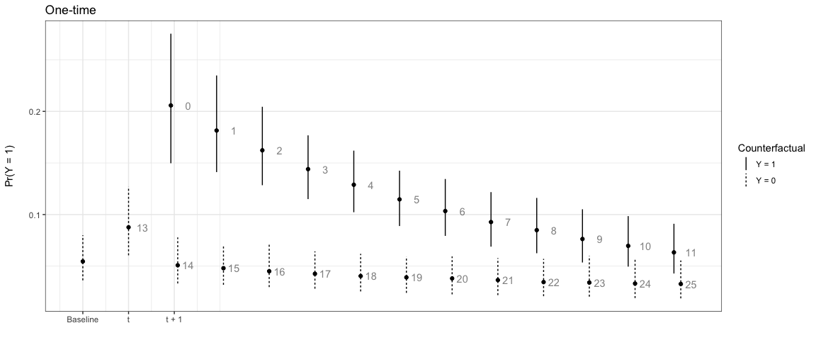

We can also have the counterfactual effect last for short periods of time and simulate the effect if another event occurs:

# Temporary
sim3 <- plte_builder(obj = m1, obj_tvar = 'spell_time', cf_duration = 4,
                     cf = counterfactual, t_points = c(13, 25))

plte_plot(sim3) + ggtitle('Temporary')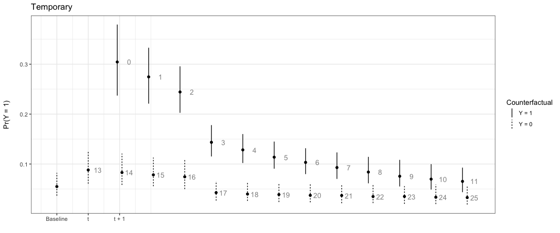

# Multiple events, permanent counter factual
sim4 <- plte_builder(obj = m1, obj_tvar = 'spell_time',
                     cf = counterfactual, t_points = c(13, 20, 25))

plte_plot(sim4) + ggtitle('Permanent, Multiple Events')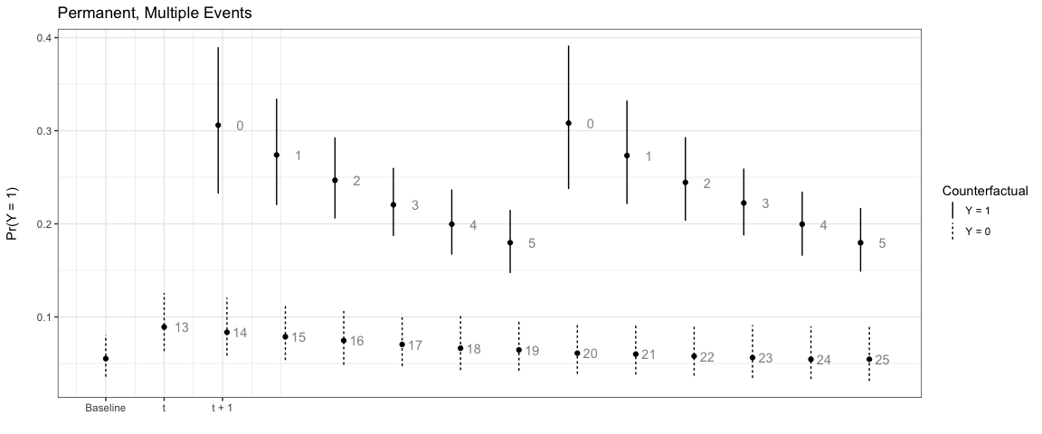

By default the baseline scenario has all covariate values fitted at 0. You can supply a custom baseline scenario in the second row of the counterfactual (cf) data frame. For example:

# Custom baseline scenario
counterfactual_baseline <- data.frame(x = c(1, 0.5))

sim5 <- plte_builder(obj = m1, obj_tvar = 'spell_time', cf_duration = 4,
                     cf = counterfactual_baseline, t_points = c(13, 25))

plte_plot(sim5) + ggtitle('Temporary, Custom Baseline')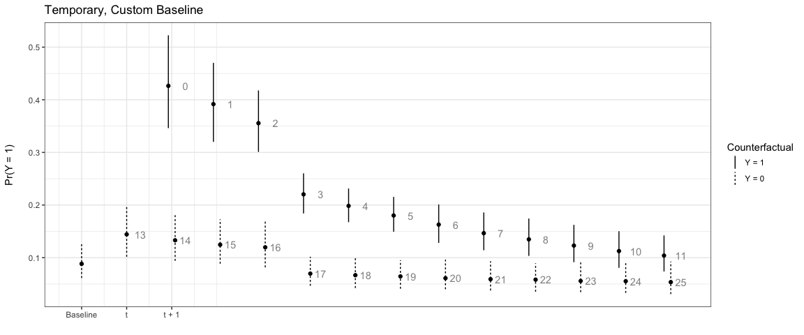

These binaries (installable software) and packages are in development.
They may not be fully stable and should be used with caution. We make no claims about them.