README

The hardware and bandwidth for this mirror is donated by METANET, the Webhosting and Full Service-Cloud Provider.
If you wish to report a bug, or if you are interested in having us mirror your free-software or open-source project, please feel free to contact us at mirror[@]metanet.ch.

pminternal: Internal Validation of Clinical Prediction Models

The goal is to offer a package that can produce bias-corrected performance measures for clinical prediction models with binary outcomes for a range of model development approaches available in R (similar to rms::validate). There are also functions for assessing prediction stability, as described in Riley and Collins (2023).

install.packages("pminternal") # cran
# or 
devtools::install_github("stephenrho/pminternal") # development

Example

In the example below we use bootstrapping to correct performance measures for a glm via calculation of ‘optimism’ (see vignette("pminternal"), vignette("validate-examples"), and vignette("missing-data") for more examples):

library(pminternal)

# make some data
set.seed(2345)
n <- 800
p <- 10

X <- matrix(rnorm(n*p), nrow = n, ncol = p)
LP <- -1 + apply(X[, 1:5], 1, sum) # first 5 variables predict outcome
y <- rbinom(n, 1, plogis(LP))

dat <- data.frame(y, X)

# fit a model
mod <- glm(y ~ ., data = dat, family = "binomial")

# calculate bootstrap optimism corrected performance measures
(val <- validate(fit = mod, method = "boot_optimism", B = 100))
#> It is recommended that B >= 200 for bootstrap validation
#>           apparent optimism corrected   n
#> C           0.8567   0.0093    0.8474 100
#> Brier       0.1423  -0.0054    0.1477 100
#> Intercept   0.0000   0.0175   -0.0175 100
#> Slope       1.0000   0.0529    0.9471 100
#> Eavg        0.0045  -0.0048    0.0093 100
#> E50         0.0039  -0.0050    0.0089 100
#> E90         0.0081  -0.0107    0.0187 100
#> Emax        0.0109  -0.0057    0.0165 100
#> ECI         0.0027  -0.0038    0.0065 100

The other available methods for calculating bias corrected performance are the simple bootstrap (boot_simple), 0.632 bootstrap optimism (.632), optimism via cross-validation (cv_optimism), and regular cross-validation (cv_average). Please see ?pminternal::validate and the references therein. Bias corrected calibration curves can also be produced (see pminternal::cal_plot). Confidence intervals can also be added via confint.

For models that cannot be supported via fit, users are able to specify their own model (model_fun) and prediction (pred_fun) functions as shown below. Note that when specifying user-defined model and prediction functions the data and outcome must also be provided. It is crucial that model_fun implements the entire model development procedure (variable selection, hyperparameter tuning, etc). For more examples, see vignette("pminternal") and vignette("validate-examples").

# fit a glm with lasso penalty
library(glmnet)
#> Loading required package: Matrix
#> Loaded glmnet 4.1-8

lasso_fun <- function(data, ...){
  y <- data$y
  x <- as.matrix(data[, which(colnames(data) != "y")])
  
  cv <- cv.glmnet(x=x, y=y, alpha=1, nfolds = 10, family="binomial")
  lambda <- cv$lambda.min
  
  glmnet(x=x, y=y, alpha = 1, lambda = lambda, family="binomial")
}

lasso_predict <- function(model, data, ...){
  y <- data$y
  x <- as.matrix(data[, which(colnames(data) != "y")])
  
  predict(model, newx = x, type = "response")[,1]
}

(val <- validate(data = dat, outcome = "y", 
                 model_fun = lasso_fun, pred_fun = lasso_predict, 
                 method = "boot_optimism", B = 100))
#> It is recommended that B >= 200 for bootstrap validation
#>           apparent optimism corrected   n
#> C            0.856   0.0070     0.849 100
#> Brier        0.143  -0.0041     0.147 100
#> Intercept    0.080   0.0191     0.061 100
#> Slope        1.155   0.0449     1.110 100
#> Eavg         0.020   0.0013     0.019 100
#> E50          0.019   0.0026     0.017 100
#> E90          0.040   0.0021     0.038 100
#> Emax         0.044   0.0145     0.029 100
#> ECI          0.053   0.0087     0.044 100

The output of validate (with method = "boot_*") can be used to produce plots for assessing the stability of model predictions (across models developed on bootstrap resamples).

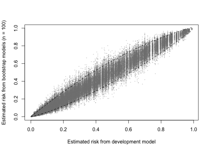
A prediction (in)stability plot shows predictions from the B (in this case 100) bootstrap models applied to the development data.

prediction_stability(val, smooth_bounds = TRUE)

A MAPE plot shows the mean absolute prediction error, which is the difference between the predicted risk from the development model and each of the B bootstrap models.

mape_stability(val)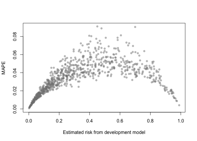

A calibration (in)stability plot depict the original calibration curve along with B calibration curves from the bootstrap models applied to the original data (y).

calibration_stability(val)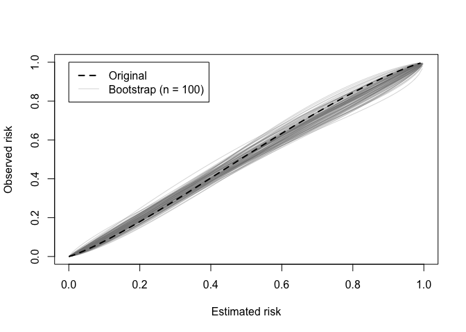

The classification instability index (CII) is the proportion of individuals that change predicted class (present/absent, 1/0) when predicted risk is compared to some threshold. For example, a patient predicted to be in class 1 would receive a CII of 0.3 if 30% of the bootstrap models led to a predicted class of 0.

classification_stability(val, threshold = .4)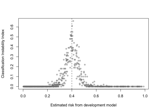

Decision curves implied by the original and bootstrap models can also be plotted.

dcurve_stability(val)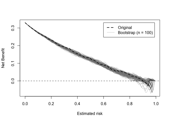

These binaries (installable software) and packages are in development.
They may not be fully stable and should be used with caution. We make no claims about them.