The hardware and bandwidth for this mirror is donated by METANET, the Webhosting and Full Service-Cloud Provider.
If you wish to report a bug, or if you are interested in having us mirror your free-software or open-source project, please feel free to contact us at mirror[@]metanet.ch.
The R package rdlearn implements the safe policy
learning under regression discontinuity designs with multiple
cutoffs of Zhang et al. (2022). It provides functions to learn
improved treatment assignment rules (cutoffs) which are guaranteed to
yield no worse overall outcomes than the existing cutoffs.
This document demonstrates how to use the main functions of
rdlearn. For the replication of the empirical results of
Zhang et al. (2022), please refer to the vignette.
The rdlearn package for R can be downloaded using
(requires previous installation of the remotes
package).
Install the latest release from CRAN:
remotes::packages("rdlearn")Install the development version from GitHub:
remotes::install_github("kkawato/rdlearn")Load the package after the installation is complete.
library(rdlearn)We can download the acces dataset and apply the proposed
methodology to the ACCES (Access with Quality to Higher Education)
program, a national-level subsidized loan initiative in Colombia.
The acces dataset includes four columns. The
elig column contains the outcome
(eligibility for the ACCES program (1: eligible; 0: not eligible). The
saber11 column contains running variable
(position scores from the SABER 11 exam). The cutoff column
contains the eligibility cutoff for each department,
and the department column contains the names of the
departments.
library(rdlearn)

# Load acces data
data(acces)
head(acces)
#> # A tibble: 6 × 4
#>    elig saber11 cutoff department
#>   <dbl>   <dbl>  <dbl> <chr>
#> 1     1      -2   -729 ANTIOQUIA
#> 2     1      -5   -729 ANTIOQUIA
#> 3     1     -11   -729 ANTIOQUIA
#> 4     1     -12   -729 ANTIOQUIA
#> 5     1     -14   -729 ANTIOQUIA
#> 6 1 -15 -729 ANTIOQUIAFirst, we demonstrate how to output a summary of the dataset, which includes local treatment effect estimates at the baseline cutoffs (such as Table 1 in Zhang et al. (2022)). This can be done as follows:
rdestimate_result <- rdestimate(
  y = "elig",
  x = "saber11",
  c = "cutoff",
  group_name = "department",
  data = acces
)
print(rdestimate_result)
#>                 Group Sample_size Baseline_cutoff RD_Estimate   se p_value
#> 1           MAGDALENA         214            -828        0.55 0.41   0.177
#> 2          LA GUAJIRA         209            -824        0.57 0.31   0.062
#> 3             BOLIVAR         646            -786        0.00 0.21   0.982
#> 4             CAQUETA         238            -779        0.56 0.35   0.107
#> 5               CAUCA         322            -774        0.02 0.78   0.977
#> 6             CORDOBA         500            -764       -0.63 0.26   0.014
#> 7               CESAR         211            -758        0.53 0.37   0.160
#> 8               SUCRE         469            -755        0.21 0.11   0.049
#> 9           ATLANTICO         448            -754        0.81 0.15   0.000
#> 10             ARAUCA         214            -753       -0.70 1.11   0.526
#> 11    VALLE DEL CAUCA         454            -732        0.61 0.16   0.000
#> 12          ANTIOQUIA         416            -729        0.70 0.21   0.001
#> 13 NORTE DE SANTANDER         233            -723       -0.08 0.43   0.858
#> 14           PUTUMAYO         236            -719       -0.47 0.79   0.556
#> 15             TOLIMA         347            -716        0.12 0.31   0.687
#> 16              HUILA         406            -695        0.06 0.23   0.797
#> 17             NARINO         463            -678        0.08 0.19   0.677
#> 18       CUNDINAMARCA         403            -676        0.12 0.81   0.882
#> 19          RISARALDA         263            -672        0.41 0.42   0.330
#> 20            QUINDIO         215            -660       -0.03 0.11   0.824
#> 21          SANTANDER         437            -632        0.74 0.25   0.003
#> 22             BOYACA         362            -618        0.48 0.36   0.187
#> 23   DISTRITO CAPITAL         539            -559        0.66 0.14   0.000
This provides basic information, including the sample size and baseline cutoff for each group, as well as the RD treatment effect and standard error. RD treatment effects marked with an asterisk (**) are significant at the 5% level.
Next, we show how to obtain the safe cutoffs by the proposed algorithm. We use the simulation data B in the Appendix D of Zhang et al. (2022). For the replication of the paper, please refer to the vignette.
Safe cutoffs can be learned as follows:
set.seed(1234)
data(simdata_B)
head(simdata_B)
#>           Y         X    C
#> 1 0.5820340 -218.9555 -571
#> 2 1.0034521 -775.4533 -571
#> 3 0.4432716 -139.2869 -571
#> 4 0.5288705 -613.2297 -571
#> 5 0.3053146 -124.8751 -571
#> 6 1.0728329 -410.1478 -571
rdlearn_result <- rdlearn(
data = simdata_B,
y = "Y",
x = "X",
c = "C",
fold = 2,
M = c(0, 1),
cost = 0,
trace = FALSE
)
summary(rdlearn_result)
#>
#> ── Basic Information ───────────────────────────────────────────────────────────
#> Group Sample_size Baseline_cutoff RD_Estimate se p_value
#> 1 Group1 273 -850 0.17 0.13 0.188
#> 2 Group2 727 -571 0.14 0.09 0.108
#>
#> ── Safe Cutoffs and Original Cutoff ────────────────────────────────────────────
#> original M=0,C=0 M=1,C=0
#> Group1 -850 -847.6996 -847.6996
#> Group2 -571 -780.9048 -633.7570
#>
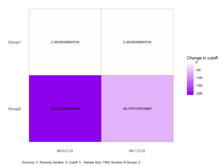
#> ── Numerical Difference of Cutoffs ─────────────────────────────────────────────
#> M=0,C=0 M=1,C=0
#> Group1 2.300363 2.300363
#> Group2 -209.904807 -62.757016
#>
#> ── Measures of Difference ──────────────────────────────────────────────────────
#> M=0,C=0 M=1,C=0
#> l1 106.1026 32.52869
#> l2 148.4340 44.40571
#> max 209.9048 62.75702plot(rdlearn_result, opt = "dif")
This plot shows the cutoff changes relative to the baseline for each
department under different smoothness multiplicative factors
(M).
The main function here is rdlearn. The arguments include
data for the dataset, y for
the column name of outcome, x for the
column name of running variable, c for the
column name of cutoff, and group_name for
the column name of group. These arguments specify the
data we analyze. The fold argument specifies the
number of folds for cross-fitting.
For sensitivity analysis, the M argument specifies
the multiplicative smoothness factor and
cost specifies the treatment cost.
For an rdlearn_result object obtained by
rdlearn, we can use summary to display the RD
estimates, the obtained safe cutoffs, and the differences between the
safe and original cutoffs.
The plot function provides a clear visualization of the
safe cutoffs. Using plot(result, opt = "safe") shows
the obtained safe cutoffs, while
plot(result,opt = "dif") shows the differences
between the safe and original cutoffs.
The trace argument can be set to TRUE to
show progress during the learning process.
Next, we implement another sensitivity analysis.
In the case of Zhang et al. (2022), we assume the utility function \(u(y, w) = y - C \times w\), where \(y\) is a binary outcome (representing the utility gain from enrollment), \(C\) is a cost parameter ranging from 0 to 1, and \(w\) is a binary treatment indicator (representing the offering of a loan). To explore the trade-off between cost and utility, we conduct a sensitivity analysis for the cost parameter: \(C\).
We use the sens function with the
rdlearn_result object as follows:
sens_result <- sens(
  rdlearn_result,
  M = 1,
  cost = c(0, 1),
  trace = FALSE)
plot(sens_result, opt = "dif")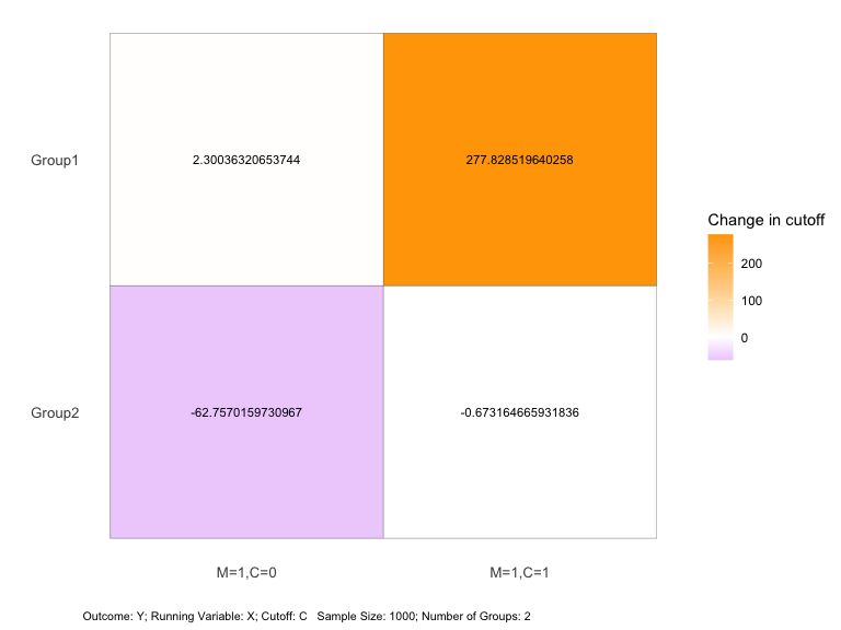
This plot shows the cutoff change relative to the baseline for each
department under different values of cost.
If the learning process has already been implemented and the
rdlearn_result object is available, the sens
function can be used to modify parameters specifically for sensitivity
analysis.
Zhang, Y., Ben-Michael, E. and Imai, K. (2022) ‘Safe Policy Learning under Regression Discontinuity Designs with Multiple Cutoffs’, arXiv [stat.ME]. Available at: http://arxiv.org/abs/2208.13323.
Melguizo, T., F. Sanchez, and T. Velasco (2016). Credit for low-income students and access to and academic performance in higher education in Colombia: A regression discontinuity approach. World Development, 80, 61–77.
These binaries (installable software) and packages are in development.
They may not be fully stable and should be used with caution. We make no claims about them.