
The hardware and bandwidth for this mirror is donated by METANET, the Webhosting and Full Service-Cloud Provider.
If you wish to report a bug, or if you are interested in having us mirror your free-software or open-source project, please feel free to contact us at mirror[@]metanet.ch.

The goal of rmacrostrat is to streamline and improve
accessibility to the geological database Macrostrat. The package provides
functionality for querying the database via the dedicated application
programming interface (API) and retrieving various geological data
(e.g., lithostratigraphic units) and definitions/metadata associated
with those data and Macrostrat more broadly.
The stable version of rmacrostrat can be installed from
CRAN using:
install.packages("rmacrostrat")You can install the development version of rmacrostrat
from GitHub with:
# install.packages("devtools")
devtools::install_github("palaeoverse/rmacrostrat")A minimal example of getting and plotting a stratigraphic column for the San Juan Basin:
# Load packages
library(rmacrostrat)
library(ggplot2)
library(ggrepel)
library(deeptime)
# Get the column definition of the San Juan Basin
column_def <- def_columns(column_name = "San Juan Basin")
# Using the column ID, retrieve all units of Cretaceous age
san_juan_units <- get_units(column_id = column_def$col_id,
                            interval_name = "Cretaceous")
# Specify x_min and x_max in dataframe
san_juan_units$x_min <- 0
san_juan_units$x_max <- 1
# Tweak values for overlapping units
san_juan_units$x_max[10] <- 0.5
san_juan_units$x_min[11] <- 0.5
# Add midpoint age for plotting
san_juan_units$m_age <- (san_juan_units$b_age +
                           san_juan_units$t_age) / 2
# Standardize and correct unit names according to USGS Geolex
san_juan_units$unit_name <- gsub(pattern = "Kirkland",
                                 replacement = "Kirtland",
                                 x = san_juan_units$unit_name)
san_juan_units$unit_name <- gsub(pattern = "Graneros Mbr",
                                 replacement = "Graneros Shale Mbr",
                                 x = san_juan_units$unit_name)
san_juan_units$unit_name <- gsub(pattern = "Sanostee Mbr",
                                 replacement = "Sanastee Sandstone Mbr",
                                 x = san_juan_units$unit_name)
# Plot stratigraphic column
ggplot(san_juan_units, aes(ymin = b_age, ymax = t_age,
                           xmin = x_min, xmax = x_max)) +
  # Plot units, colored by rock type
  geom_rect(fill = san_juan_units$color, color = "black") +
  # Add text labels
  geom_text_repel(aes(x = x_max, y = m_age, label = unit_name),
                  box.padding = 0.1, nudge_x = 3,
                  size = 3.5) +
  # Reverse direction of y-axis
  scale_y_reverse(limits = c(145, 66), n.breaks = 10,
                  name = "Time (Ma)") +
  # Theming
  theme_classic() +
  theme(legend.position = "none",
        axis.line.x = element_blank(),
        axis.title.x = element_blank(),
        axis.text.x = element_blank(),
        axis.ticks.x = element_blank()) +
  # Add geological time scale
  coord_geo(pos = "left", dat = list("stages"), rot = 90)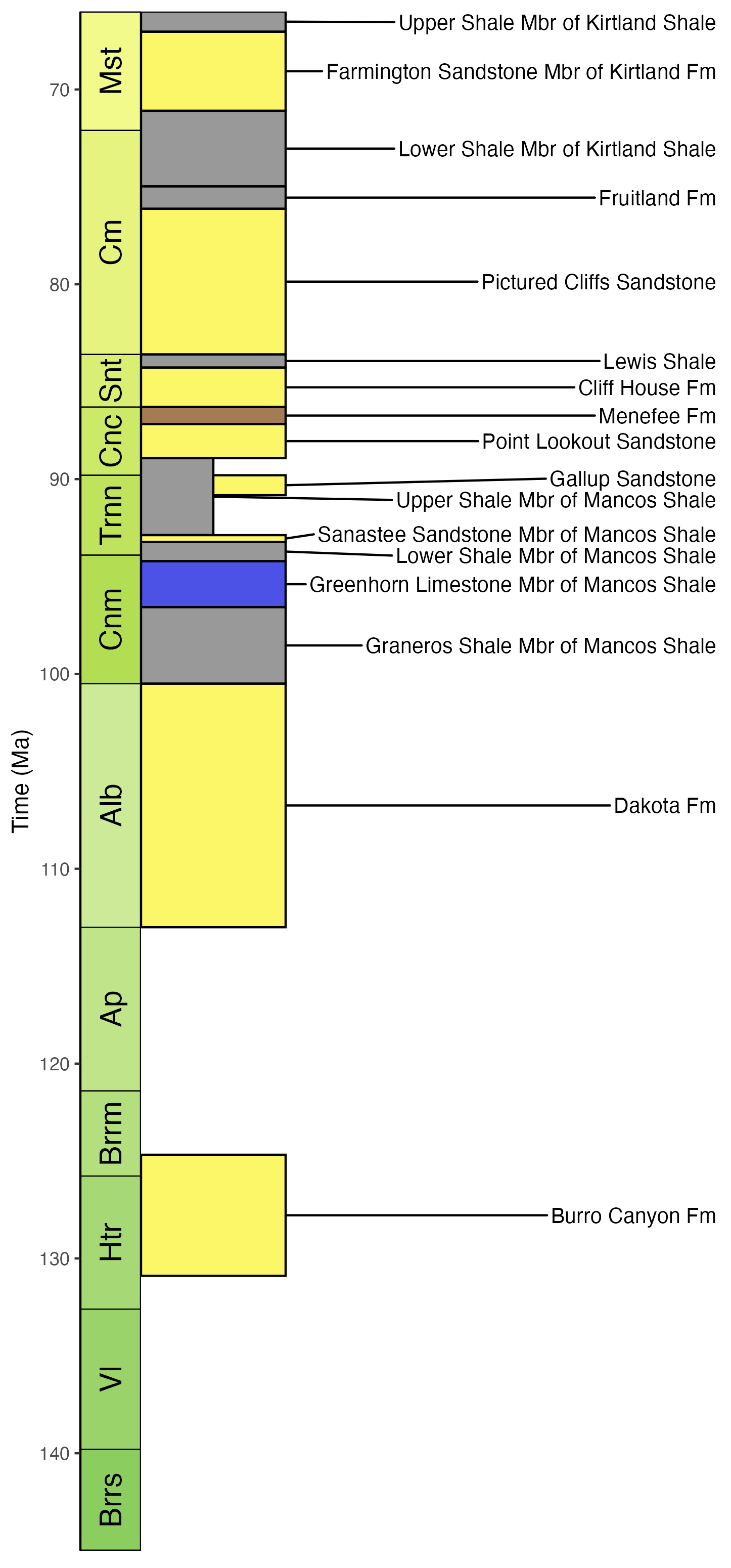
A minimal example of getting and plotting outcrop data for the Hell Creek formation:
# Load libraries
library(rmacrostrat)
library(ggplot2)
library(ggspatial)
# Get data for the chosen formation
hc_def <- def_strat_names(strat_name = "Hell Creek", rank = "Fm")
# Get spatial outcrop data for the formation
hc <- get_map_outcrop(strat_name_id = hc_def$strat_name_id, sf = TRUE)
# Plot the map
ggplot() +
  geom_sf(data = hc, fill = "#C7622B", lwd = 0) +
  coord_sf(xlim = c(-112, -97), ylim = c(44, 50)) +
  annotation_north_arrow(location = "br",
                         pad_y = unit(0.75, "cm"),
                         height = unit(1, "cm"), width = unit(1, "cm")) +
  annotation_scale(location = "br", width_hint = 0.3) +
  theme_bw()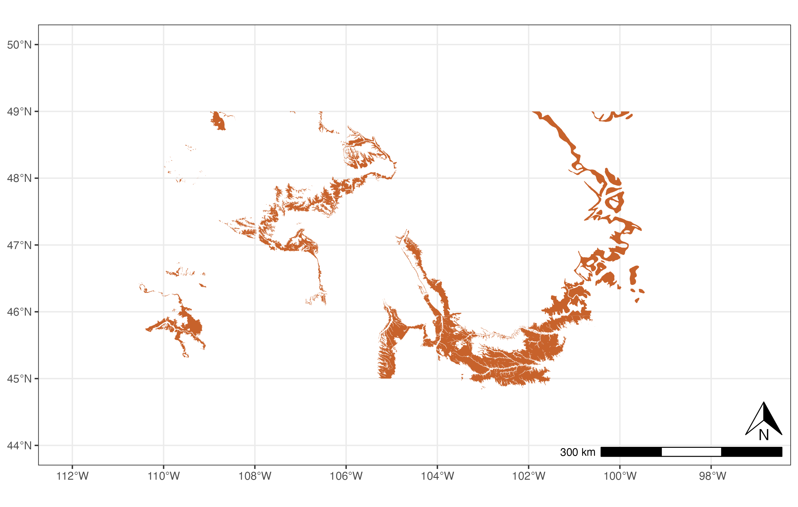
A minimal example of getting and plotting the number of marine units through time for North America:
# Load libraries
library(rmacrostrat)
library(ggplot2)
library(deeptime)
# Get all carbonate units for North America
units <- get_units(environ_class = "marine",
                   interval_name = "Phanerozoic",
                   project_id = 1)
# Add mid age for units
units$mid_age <- (units$b_age + units$t_age) / 2
# Plot data
ggplot(units, aes(x = mid_age)) +
  geom_histogram(binwidth = 10, center = 5,
                 color = "black", fill = "#add8e6") +
  scale_y_continuous("Number of marine units") +
  scale_x_reverse("Time (Ma)", limits = c(538.8, 0)) +
  theme_bw() +
  theme(legend.title = element_blank(),
        legend.position.inside = c(0.1, 0.9)) +
  coord_geo()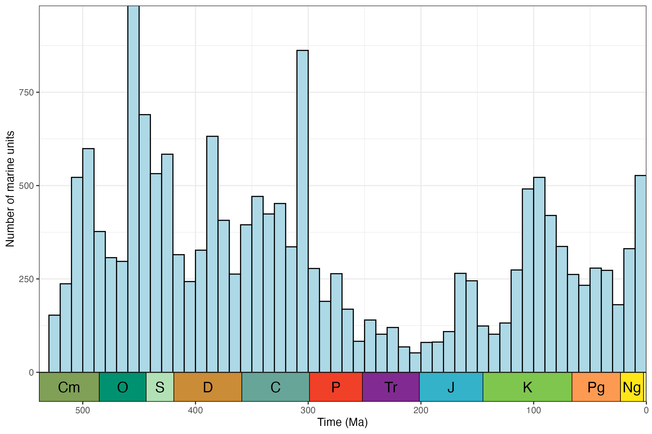
Extensive example usage of rmacrostrat is provided in
the package vignettes/tutorials. These can be accessed online or in R
via:
browseVignettes(package = "rmacrostrat")If you are interested in contributing to the rmacrostrat
R package, you can do so by following these guidelines.
We have also adopted a set of standards
and structure to broadly follow for contributing to Palaeoverse R
packages. If you would like to contribute to rmacrostrat,
we strongly advise reading this document.
As with any community project, society, or meeting we feel it is
important to established some expectations of behaviour in the
rmacrostrat community. Please read our code of
conduct, and reach out if you ever face any issues. Everyone has the
right to live and work in a harassment-free environment.
If you use the rmacrostrat R package in your work,
please cite as:
Jones, L.A., Dean, C.D., Gearty, W., and Allen, B.J. 2024. rmacrostrat: An R package for accessing and retrieving data from the Macrostrat geological database. EarthArXiv. doi: 10.31223/X5XX37.

Hexlogo by Miranta Kouvari
These binaries (installable software) and packages are in development.
They may not be fully stable and should be used with caution. We make no claims about them.