The hardware and bandwidth for this mirror is donated by METANET, the Webhosting and Full Service-Cloud Provider.
If you wish to report a bug, or if you are interested in having us mirror your free-software or open-source project, please feel free to contact us at mirror[@]metanet.ch.

sentimentr is designed to quickly calculate text polarity sentiment in the English language at the sentence level and optionally aggregate by rows or grouping variable(s).
sentimentr is a response to my own needs with
sentiment detection that were not addressed by the current
R tools. My own polarity function in the
qdap package is slower on larger data sets. It is a
dictionary lookup approach that tries to incorporate weighting for
valence shifters (negation and amplifiers/deamplifiers). Matthew Jockers
created the syuzhet
package that utilizes dictionary lookups for the Bing, NRC, and Afinn
methods as well as a custom dictionary. He also utilizes a wrapper for
the Stanford
coreNLP which uses much more sophisticated analysis. Jocker’s
dictionary methods are fast but are more prone to error in the case of
valence shifters. Jocker’s addressed
these critiques explaining that the method is good with regard to
analyzing general sentiment in a piece of literature. He points to the
accuracy of the Stanford detection as well. In my own work I need better
accuracy than a simple dictionary lookup; something that considers
valence shifters yet optimizes speed which the Stanford’s parser does
not. This leads to a trade off of speed vs. accuracy. Simply,
sentimentr attempts to balance accuracy and speed.
So what does sentimentr do that other packages don’t and why does it matter?
sentimentr attempts to take into account valence shifters (i.e., negators, amplifiers (intensifiers), de-amplifiers (downtoners), and adversative conjunctions) while maintaining speed. Simply put, sentimentr is an augmented dictionary lookup. The next questions address why it matters.
So what are these valence shifters?
A negator flips the sign of a polarized word (e.g., “I do not like it.”). See
lexicon::hash_valence_shifters[y==1]for examples. An amplifier (intensifier) increases the impact of a polarized word (e.g., “I really like it.”). Seelexicon::hash_valence_shifters[y==2]for examples. A de-amplifier (downtoner) reduces the impact of a polarized word (e.g., “I hardly like it.”). Seelexicon::hash_valence_shifters[y==3]for examples. An adversative conjunction overrules the previous clause containing a polarized word (e.g., “I like it but it’s not worth it.”). Seelexicon::hash_valence_shifters[y==4]for examples.
Do valence shifters really matter?
Well valence shifters affect the polarized words. In the case of negators and adversative conjunctions the entire sentiment of the clause may be reversed or overruled. So if valence shifters occur fairly frequently a simple dictionary lookup may not be modeling the sentiment appropriately. You may be wondering how frequently these valence shifters co-occur with polarized words, potentially changing, or even reversing and overruling the clause’s sentiment. The table below shows the rate of sentence level co-occurrence of valence shifters with polarized words across a few types of texts.
| Text | Negator | Amplifier | Deamplifier | Adversative |
|---|---|---|---|---|
| Cannon reviews | 21% | 23% | 8% | 12% |
| 2012 presidential debate | 23% | 18% | 1% | 11% |
| Trump speeches | 12% | 14% | 3% | 10% |
| Trump tweets | 19% | 18% | 4% | 4% |
| Dylan songs | 4% | 10% | 0% | 4% |
| Austen books | 21% | 18% | 6% | 11% |
| Hamlet | 26% | 17% | 2% | 16% |
Indeed negators appear ~20% of the time a polarized word appears in a sentence. Conversely, adversative conjunctions appear with polarized words ~10% of the time. Not accounting for the valence shifters could significantly impact the modeling of the text sentiment.
The script to replicate the frequency analysis, shown in the table above, can be accessed via:
val_shift_freq <- system.file("the_case_for_sentimentr/valence_shifter_cooccurrence_rate.R", package = "sentimentr")
file.copy(val_shift_freq, getwd())There are two main functions (top 2 in table below) in sentimentr with several helper functions summarized in the table below:
| Function | Description |
|---|---|
sentiment
|
Sentiment at the sentence level |
sentiment_by
|
Aggregated sentiment by group(s) |
profanity
|
Profanity at the sentence level |
profanity_by
|
Aggregated profanity by group(s) |
emotion
|
Emotion at the sentence level |
emotion_by
|
Aggregated emotion by group(s) |
uncombine
|
Extract sentence level sentiment from sentiment_by
|
get_sentences
|
Regex based string to sentence parser (or get sentences from
sentiment/sentiment_by)
|
replace_emoji
|
repalcement |
replace_emoticon
|
Replace emoticons with word equivalent |
replace_grade
|
Replace grades (e.g., "A+") with word equivalent |
replace_internet_slang
|
replacment |
replace_rating
|
Replace ratings (e.g., "10 out of 10", "3 stars") with word equivalent |
as_key
|
Coerce a data.frame lexicon to a polarity hash key
|
is_key
|
Check if an object is a hash key |
update_key
|
Add/remove terms to/from a hash key |
highlight
|
Highlight positive/negative sentences as an HTML document |
general_rescale
|
Generalized rescaling function to rescale sentiment scoring |
sentiment_attribute
|
Extract the sentiment based attributes from a text |
validate_sentiment
|
Validate sentiment score sign against known results |
The equation below describes the augmented dictionary method of sentimentr that may give better results than a simple lookup dictionary approach that does not consider valence shifters. The equation used by the algorithm to assign value to polarity of each sentence fist utilizes a sentiment dictionary (e.g., Jockers, (2017)) to tag polarized words. Each paragraph (pi = {s1, s2, …, sn}) composed of sentences, is broken into element sentences (si, j = {w1, w2, …, wn}) where w are the words within sentences. Each sentence (sj) is broken into a an ordered bag of words. Punctuation is removed with the exception of pause punctuations (commas, colons, semicolons) which are considered a word within the sentence. I will denote pause words as *c**w* (comma words) for convenience. We can represent these words as an i,j,k notation as wi, j, k. For example w3, 2, 5 would be the fifth word of the second sentence of the third paragraph. While I use the term paragraph this merely represent a complete turn of talk. For example it may be a cell level response in a questionnaire composed of sentences.
The words in each sentence (wi, j, k) are searched and compared to a dictionary of polarized words (e.g., a combined and augmented version of Jocker’s (2017) [originally exported by the syuzhet package] & Rinker’s augmented Hu & Liu (2004) dictionaries in the lexicon package). Positive (wi, j, k+) and negative (wi, j, k−) words are tagged with a +1 and −1 respectively (or other positive/negative weighting if the user provides the sentiment dictionary). I will denote polarized words as *p**w* for convenience. These will form a polar cluster (ci, j, l) which is a subset of the a sentence (ci, j, l ⊆ si, j).
The polarized context cluster
(ci, j, l) of words is
pulled from around the polarized word (pw) and defaults
to 4 words before and two words after pw to be
considered as valence shifters. The cluster can be represented as
(ci, j, l = {pwi, j, k − nb, …, pwi, j, k, …, pwi, j, k − na}),
where nb & *n**a* are the parameters
n.before and n.after set by the user. The
words in this polarized context cluster are tagged as neutral
(wi, j, k0),
negator
(wi, j, kn),
amplifier [intensifier]
(wi, j, ka),
or de-amplifier [downtoner]
(wi, j, kd).
Neutral words hold no value in the equation but do affect word count
(n). Each polarized word is then weighted (w) based on
the weights from the polarity_dt argument and then further
weighted by the function and number of the valence shifters directly
surrounding the positive or negative word (pw). Pause
(cw) locations (punctuation that denotes a pause
including commas, colons, and semicolons) are indexed and considered in
calculating the upper and lower bounds in the polarized context cluster.
This is because these marks indicate a change in thought and words prior
are not necessarily connected with words after these punctuation marks.
The lower bound of the polarized context cluster is constrained to
max{pwi, j, k − nb, 1, max{cwi, j, k < pwi, j, k}}
and the upper bound is constrained to
min{pwi, j, k + na, wi, jn, min{cwi, j, k > pwi, j, k}}
where wi, jn is the
number of words in the sentence.
The core value in the cluster, the polarized word is acted upon by valence shifters. Amplifiers increase the polarity by 1.8 (.8 is the default weight (z)). Amplifiers (wi, j, ka) become de-amplifiers if the context cluster contains an odd number of negators (wi, j, kn). De-amplifiers work to decrease the polarity. Negation (wi, j, kn) acts on amplifiers/de-amplifiers as discussed but also flip the sign of the polarized word. Negation is determined by raising −1 to the power of the number of negators (wi, j, kn) plus 2. Simply, this is a result of a belief that two negatives equal a positive, 3 negatives a negative, and so on.
The adversative conjunctions (i.e., ‘but’, ‘however’, and ‘although’) also weight the context cluster. An adversative conjunction before the polarized word (wadversative conjunction, …, wi, j, kp) up-weights the cluster by 1 + z2 * {|wadversative conjunction|,…,wi, j, kp} (.85 is the default weight (z2) where |wadversative conjunction| are the number of adversative conjunctions before the polarized word). An adversative conjunction after the polarized word down-weights the cluster by 1 + {wi, j, kp, …, |wadversative conjunction|* − 1}*z2. This corresponds to the belief that an adversative conjunction makes the next clause of greater values while lowering the value placed on the prior clause.
The researcher may provide a weight (z) to be utilized with amplifiers/de-amplifiers (default is .8; de-amplifier weight is constrained to −1 lower bound). Last, these weighted context clusters (ci, j, l) are summed (c′i, j) and divided by the square root of the word count (√wi, *j**n) yielding an unbounded polarity score (δi, j*) for each sentence.
δij = c’ij/√wijn
Where:
c′i, j = ∑((1 + wamp + wdeamp)⋅wi, j, kp(−1)2 + wneg)
wamp = ∑(wneg ⋅ (z ⋅ wi, j, ka))
wdeamp = max(wdeamp′, −1)
wdeamp′ = ∑(z(−wneg ⋅ wi, j, ka + wi, j, kd))
wb = 1 + z2 * wb′
wb′ = ∑(|wadversative conjunction|,…,wi, j, kp, wi, j, kp, …, |wadversative conjunction|* − 1)
wneg = (∑wi, j, kn ) mod 2
To get the mean of all sentences
(si, j) within a paragraph/turn of
talk (pi) simply take the average sentiment
score
pi, δi, j
= 1/n ⋅ ∑ δi, j or use an
available weighted average (the default
average_weighted_mixed_sentiment which upweights the
negative values in a vector while also downweighting the zeros in a
vector or average_downweighted_zero which simply
downweights the zero polarity scores).
To download the development version of sentimentr:
Download the zip ball
or tar
ball, decompress and run R CMD INSTALL on it, or use
the pacman package to install the development
version:
if (!require("pacman")) install.packages("pacman")
pacman::p_load_current_gh("trinker/lexicon", "trinker/sentimentr")if (!require("pacman")) install.packages("pacman")
pacman::p_load(sentimentr, dplyr, magrittr)Here is a basic sentiment demo. Notice that the first
thing you should do is to split your text data into sentences (a process
called sentence boundary disambiguation) via the
get_sentences function. This can be handled within
sentiment (i.e., you can pass a raw character vector) but
it slows the function down and should be done one time rather than every
time the function is called. Additionally, a warning will be thrown if a
larger raw character vector is passed. The preferred workflow is to spit
the text into sentences with get_sentences before any
sentiment analysis is done.
mytext <- c(
    'do you like it?  But I hate really bad dogs',
    'I am the best friend.',
    'Do you really like it?  I\'m not a fan'
)

mytext <- get_sentences(mytext)
sentiment(mytext)

##    element_id sentence_id word_count  sentiment
## 1:          1           1          4  0.2500000
## 2:          1           2          6 -1.8677359
## 3:          2           1          5  0.5813777
## 4:          3           1          5  0.4024922
## 5:          3           2          4  0.0000000
To aggregate by element (column cell or vector element) use
sentiment_by with by = NULL.
mytext <- c(
    'do you like it?  But I hate really bad dogs',
    'I am the best friend.',
    'Do you really like it?  I\'m not a fan'
)
mytext <- get_sentences(mytext)
sentiment_by(mytext)

##    element_id word_count       sd ave_sentiment
## 1:          1         10 1.497465    -0.8088680
## 2:          2          5       NA     0.5813777
## 3:          3          9 0.284605     0.2196345
To aggregate by grouping variables use sentiment_by
using the by argument.
(out <- with(
    presidential_debates_2012,
    sentiment_by(
        get_sentences(dialogue),
        list(person, time)
    )
))

##        person   time word_count        sd ave_sentiment
##  1:     OBAMA time 1       3599 0.2535006    0.12256892
##  2:     OBAMA time 2       7477 0.2509177    0.11217673
##  3:     OBAMA time 3       7243 0.2441394    0.07975688
##  4:    ROMNEY time 1       4085 0.2525596    0.10151917
##  5:    ROMNEY time 2       7536 0.2205169    0.08791018
##  6:    ROMNEY time 3       8303 0.2623534    0.09968544
##  7:   CROWLEY time 2       1672 0.2181662    0.19455290
##  8:    LEHRER time 1        765 0.2973360    0.15473364
##  9:  QUESTION time 2        583 0.1756778    0.03197751
## 10: SCHIEFFER time 3 1445 0.2345187 0.08843478Or if you prefer a more tidy approach:
library(magrittr)
library(dplyr)

presidential_debates_2012 %>%
    dplyr::mutate(dialogue_split = get_sentences(dialogue)) %$%
    sentiment_by(dialogue_split, list(person, time))

##        person   time word_count        sd ave_sentiment
##  1:     OBAMA time 1       3599 0.2535006    0.12256892
##  2:     OBAMA time 2       7477 0.2509177    0.11217673
##  3:     OBAMA time 3       7243 0.2441394    0.07975688
##  4:    ROMNEY time 1       4085 0.2525596    0.10151917
##  5:    ROMNEY time 2       7536 0.2205169    0.08791018
##  6:    ROMNEY time 3       8303 0.2623534    0.09968544
##  7:   CROWLEY time 2       1672 0.2181662    0.19455290
##  8:    LEHRER time 1        765 0.2973360    0.15473364
##  9:  QUESTION time 2        583 0.1756778    0.03197751
## 10: SCHIEFFER time 3       1445 0.2345187    0.08843478
Note that you can skip the dplyr::mutate step by using
get_sentences on a data.frame as seen
below:
presidential_debates_2012 %>%
    get_sentences() %$%
    sentiment_by(dialogue, list(person, time))

##        person   time word_count        sd ave_sentiment
##  1:     OBAMA time 1       3599 0.2535006    0.12256892
##  2:     OBAMA time 2       7477 0.2509177    0.11217673
##  3:     OBAMA time 3       7243 0.2441394    0.07975688
##  4:    ROMNEY time 1       4085 0.2525596    0.10151917
##  5:    ROMNEY time 2       7536 0.2205169    0.08791018
##  6:    ROMNEY time 3       8303 0.2623534    0.09968544
##  7:   CROWLEY time 2       1672 0.2181662    0.19455290
##  8:    LEHRER time 1        765 0.2973360    0.15473364
##  9:  QUESTION time 2        583 0.1756778    0.03197751
## 10: SCHIEFFER time 3 1445 0.2345187 0.08843478plot(out)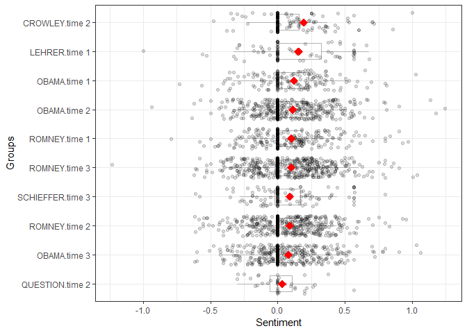
The plot method for the class sentiment
uses syuzhet’s get_transformed_values
combined with ggplot2 to make a reasonable, smoothed
plot for the duration of the text based on percentage, allowing for
comparison between plots of different texts. This plot gives the overall
shape of the text’s sentiment. The user can see
syuzhet::get_transformed_values for more details.
plot(uncombine(out))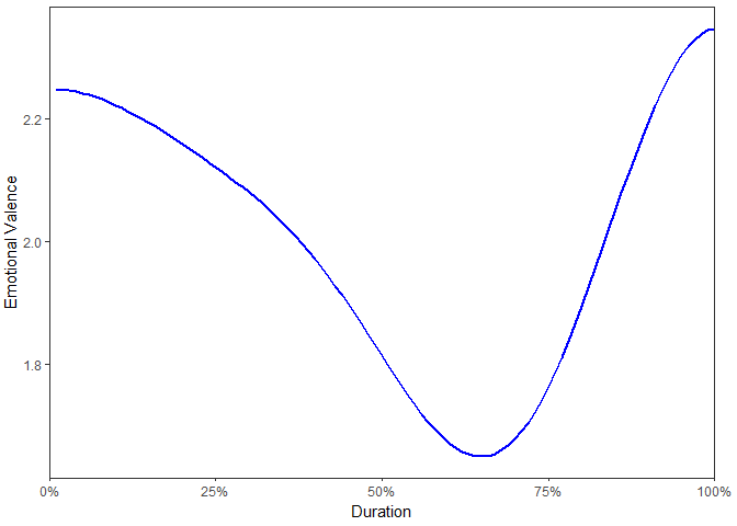
It is pretty straight forward to make or update a new dictionary
(polarity or valence shifter). To create a key from scratch the user
needs to create a 2 column data.frame, with words on the
left and values on the right (see
?lexicon::hash_sentiment_jockers_rinker &
?lexicon::hash_valence_shifters for what the values mean).
Note that the words need to be lower cased. Here I show an example
data.frame ready for key conversion:
set.seed(10)
key <- data.frame(
    words = sample(letters),
    polarity = rnorm(26),
    stringsAsFactors = FALSE
)
This is not yet a key. sentimentr provides the
is_key function to test if a table is a key.
is_key(key)

## [1] FALSE
It still needs to be data.table-ified. The
as_key function coerces a data.frame to a
data.table with the left column named x
and the right column named y. It also checks the key
against another key to make sure there is not overlap using the
compare argument. By default as_key checks
against valence_shifters_table, assuming the user is
creating a sentiment dictionary. If the user is creating a valence
shifter key then a sentiment key needs to be passed to
compare instead and set the argument
sentiment = FALSE. Below I coerce key to a
dictionary that sentimentr can use.
mykey <- as_key(key)Now we can check that mykey is a usable dictionary:
is_key(mykey)

## [1] TRUE
The key is ready for use:
sentiment_by("I am a human.", polarity_dt = mykey)

##    element_id word_count sd ave_sentiment
## 1:          1          4 NA    -0.7594893
You can see the values of a key that correspond to a word using data.table syntax:
mykey[c("a", "b")][[2]]

## [1] -0.2537805 -0.1951504
Updating (adding or removing terms) a key is also useful. The
update_key function allows the user to add or drop terms
via the x (add a data.frame) and
drop (drop a term) arguments. Below I drop the “a” and “h”
terms (notice there are now 24 rows rather than 26):
mykey_dropped <- update_key(mykey, drop = c("a", "h"))
nrow(mykey_dropped)

## [1] 24

sentiment_by("I am a human.", polarity_dt = mykey_dropped)

##    element_id word_count sd ave_sentiment
## 1:          1          4 NA     -0.632599
Next I add the terms “dog” and “cat” as a data.frame
with sentiment values:
mykey_added <- update_key(mykey, x = data.frame(x = c("dog", "cat"), y = c(1, -1)))

## Warning in as_key(x, comparison = comparison, sentiment = sentiment): Column 1 was a factor...
## Converting to character.

nrow(mykey_added)

## [1] 28

sentiment("I am a human. The dog.  The cat", polarity_dt = mykey_added)

##    element_id sentence_id word_count  sentiment
## 1:          1           1          4 -0.7594893
## 2:          1           2          2  0.7071068
## 3:          1           3          2 -0.7071068
Annie
Swafford critiqued Jocker’s approach to sentiment and gave the
following examples of sentences (ase for Annie Swafford
example). Here I test each of Jocker’s 4 dictionary approaches (syuzhet,
Bing, NRC, Afinn), his Stanford wrapper (note I use my own GitHub Stanford wrapper
package based off of Jocker’s approach as it works more reliably on
my own Windows machine), the RSentiment
package, the lookup based SentimentAnalysis
package, the meanr
package (written in C level code), and my own algorithm with default
combined Jockers (2017) & Rinker’s augmented Hu & Liu (2004)
polarity lexicons as well as Hu & Liu (2004) and Baccianella, Esuli
and Sebastiani’s (2010) SentiWord lexicons available from the lexicon
package.
if (!require("pacman")) install.packages("pacman")
pacman::p_load_gh("trinker/sentimentr", "trinker/stansent", "sfeuerriegel/SentimentAnalysis", "wrathematics/meanr")
pacman::p_load(syuzhet, qdap, microbenchmark, RSentiment)

ase <- c(
    "I haven't been sad in a long time.",
    "I am extremely happy today.",
    "It's a good day.",
    "But suddenly I'm only a little bit happy.",
    "Then I'm not happy at all.",
    "In fact, I am now the least happy person on the planet.",
    "There is no happiness left in me.",
    "Wait, it's returned!",
    "I don't feel so bad after all!"
)

syuzhet <- setNames(as.data.frame(lapply(c("syuzhet", "bing", "afinn", "nrc"),
    function(x) get_sentiment(ase, method=x))), c("jockers", "bing", "afinn", "nrc"))

SentimentAnalysis <- apply(analyzeSentiment(ase)[c('SentimentGI', 'SentimentLM', 'SentimentQDAP') ], 2, round, 2)
colnames(SentimentAnalysis) <- gsub('^Sentiment', "SA_", colnames(SentimentAnalysis))

left_just(data.frame(
    stanford = sentiment_stanford(ase)[["sentiment"]],
    sentimentr_jockers_rinker = round(sentiment(ase, question.weight = 0)[["sentiment"]], 2),
    sentimentr_jockers = round(sentiment(ase, lexicon::hash_sentiment_jockers, question.weight = 0)[["sentiment"]], 2),
    sentimentr_huliu = round(sentiment(ase, lexicon::hash_sentiment_huliu, question.weight = 0)[["sentiment"]], 2),
    sentimentr_sentiword = round(sentiment(ase, lexicon::hash_sentiment_sentiword, question.weight = 0)[["sentiment"]], 2),
    RSentiment = calculate_score(ase),
    SentimentAnalysis,
    meanr = score(ase)[['score']],
    syuzhet,
    sentences = ase,
    stringsAsFactors = FALSE
), "sentences")

[1] "Processing sentence: i have not been sad in a long time"
[1] "Processing sentence: i am extremely happy today"
[1] "Processing sentence: its a good day"
[1] "Processing sentence: but suddenly im only a little bit happy"
[1] "Processing sentence: then im not happy at all"
[1] "Processing sentence: in fact i am now the least happy person on the planet"
[1] "Processing sentence: there is no happiness left in me"
[1] "Processing sentence: wait its returned"
[1] "Processing sentence: i do not feel so bad after all"

  stanford sentimentr_jockers_rinker sentimentr_jockers sentimentr_huliu
1     -0.5                      0.18               0.18             0.35
2        1                       0.6                0.6              0.8
3      0.5                      0.38               0.38              0.5
4     -0.5                         0                  0                0
5     -0.5                     -0.31              -0.31            -0.41
6     -0.5                      0.04               0.04             0.06
7     -0.5                     -0.28              -0.28            -0.38
8        0                     -0.14              -0.14                0
9     -0.5                      0.28               0.28             0.38
  sentimentr_sentiword RSentiment SA_GI SA_LM SA_QDAP meanr jockers bing
1                 0.18          1 -0.25     0   -0.25    -1    -0.5   -1
2                 0.65          1  0.33  0.33       0     1    0.75    1
3                 0.32          1   0.5   0.5     0.5     1    0.75    1
4                    0          0     0  0.25    0.25     1    0.75    1
5                -0.56         -1     1     1       1     1    0.75    1
6                 0.11          1  0.17  0.17    0.33     1    0.75    1
7                -0.05          1   0.5   0.5     0.5     1    0.75    1
8                -0.14         -1     0     0       0     0   -0.25    0
9                 0.24          0 -0.33 -0.33   -0.33    -1   -0.75   -1
  afinn nrc sentences
1    -2   0 I haven't been sad in a long time.
2     3   1 I am extremely happy today.
3     3   1 It's a good day.
4     3   1 But suddenly I'm only a little bit happy.
5     3   1 Then I'm not happy at all.
6     3   1 In fact, I am now the least happy person on the planet.
7     2   1 There is no happiness left in me.
8     0  -1 Wait, it's returned!
9    -3  -1 I don't feel so bad after all!
Also of interest is the computational time used by each of these
methods. To demonstrate this I increased Annie’s examples by 100
replications and microbenchmark on a few iterations
(Stanford takes so long I didn’t extend to more). Note that if a text
needs to be broken into sentence parts syuzhet has the
get_sentences function that uses the
openNLP package, this is a time expensive task.
sentimentr uses a much faster regex based approach that
is nearly as accurate in parsing sentences with a much lower
computational time. We see that RSentiment and Stanford
take the longest time while sentimentr and
syuzhet are comparable depending upon lexicon used.
meanr is lighting fast.
SentimentAnalysis is a bit slower than other methods
but is returning 3 scores from 3 different dictionaries. I do not test
RSentiment because it causes an out of memory
error.
ase_100 <- rep(ase, 100)

stanford <- function() {sentiment_stanford(ase_100)}

sentimentr_jockers_rinker <- function() sentiment(ase_100, lexicon::hash_sentiment_jockers_rinker)
sentimentr_jockers <- function() sentiment(ase_100, lexicon::hash_sentiment_jockers)
sentimentr_huliu <- function() sentiment(ase_100, lexicon::hash_sentiment_huliu)
sentimentr_sentiword <- function() sentiment(ase_100, lexicon::hash_sentiment_sentiword)

RSentiment <- function() calculate_score(ase_100)

SentimentAnalysis <- function() analyzeSentiment(ase_100)

meanr <- function() score(ase_100)

syuzhet_jockers <- function() get_sentiment(ase_100, method="syuzhet")
syuzhet_binn <- function() get_sentiment(ase_100, method="bing")
syuzhet_nrc <- function() get_sentiment(ase_100, method="nrc")
syuzhet_afinn <- function() get_sentiment(ase_100, method="afinn")

microbenchmark(
    stanford(),
    sentimentr_jockers_rinker(),
    sentimentr_jockers(),
    sentimentr_huliu(),
    sentimentr_sentiword(),
    #RSentiment(),
    SentimentAnalysis(),
    syuzhet_jockers(),
    syuzhet_binn(),
    syuzhet_nrc(),
    syuzhet_afinn(),
    meanr(),
    times = 3
)

Unit: milliseconds
                        expr          min           lq         mean
                  stanford() 20225.158418 20609.912899 23748.607689
 sentimentr_jockers_rinker()   283.271569   283.391307   285.273047
        sentimentr_jockers()   224.436569   228.487136   235.022980
          sentimentr_huliu()   255.438460   260.156352   261.994973
      sentimentr_sentiword()  1048.496476  1060.058681  1064.804513
         SentimentAnalysis()  4267.380620  4335.857740  4369.068442
           syuzhet_jockers()   342.764273   346.408800   349.115379
              syuzhet_binn()   258.453721   267.449255   271.441450
               syuzhet_nrc()   642.814135   648.150176   653.361347
             syuzhet_afinn()   118.191289   120.576642   122.294740
                     meanr()     1.172578     1.317333     1.795786
       median          uq          max neval
 20994.667381 25510.33232 30025.997269     3
   283.511045   286.27379   289.036528     3
   232.537703   240.31619   248.094669     3
   264.874245   265.27323   265.672214     3
  1071.620886  1072.95853  1074.296176     3
  4404.334860  4419.91235  4435.489845     3
   350.053327   352.29093   354.528537     3
   276.444790   277.93532   279.425840     3
   653.486217   658.63495   663.783689     3
   122.961995   124.34647   125.730937     3
1.462088 2.10739 2.752692 3The accuracy of an algorithm weighs heavily into the decision as to what approach to take in sentiment detection. I have selected algorithms/packages that stand out as fast and/or accurate to perform benchmarking on actual data. The syuzhet package provides multiple dictionaries with a general algorithm to compute sentiment scores. Likewise, sentimentr uses a general algorithm but uses the lexicon package’s dictionaries. syuzhet provides 4 dictionaries while sentimentr uses lexicon’s 9 dictionaries and can be extended easily other dictionaries including the 4 dictionaries from the syuzhet package. meanr is a very fast algorithm. The follow visualization provides the accuracy of these approaches in comparison to Stanford’s Java based implementation of sentiment detection. The visualization is generated from testing on three reviews data sets from Kotzias, Denil, De Freitas, & Smyth (2015). These authors utilized the three 1000 element data sets from:
The data sets are hand scored as either positive or negative. The testing here uses Mean Directional Accuracy (MDA) and merely matches the sign of the algorithm to the human coded output to determine accuracy rates.
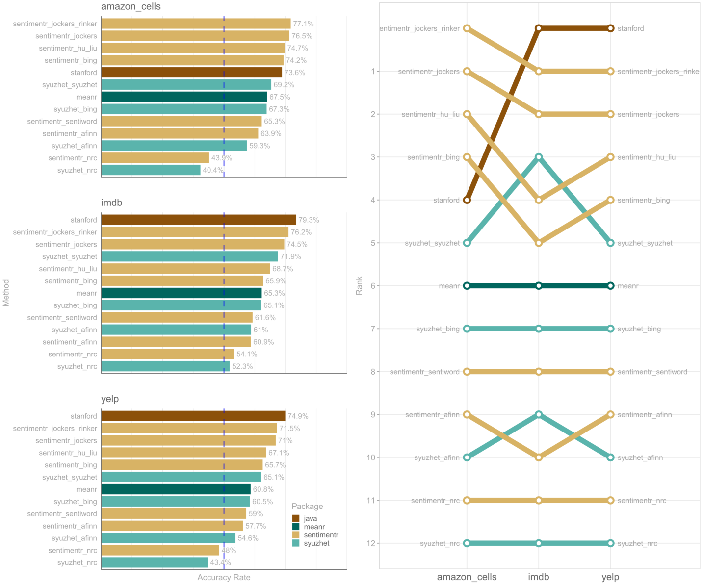
The bar graph on the left shows the accuracy rates for the various sentiment set-ups in the three review contexts. The rank plot on the right shows how the rankings for the methods varied across the three review contexts.
The take away here seems that, unsurprisingly, Stanford’s algorithm
consistently outscores sentimentr,
syuzhet, and meanr. The
sentimentr approach loaded with the Jockers’ custom
syuzhet dictionary is a top pick for speed and
accuracy. In addition to Jockers’ custom dictionary the
bing dictionary also performs well within both the
syuzhet and sentimentr algorithms.
Generally, the sentimentr algorithm out performs
syuzhet when their dictionaries are comparable.
It is important to point out that this is a small sample data set that covers a narrow range of uses for sentiment detection. Jockers’ syuzhet was designed to be applied across book chunks and it is, to some extent, unfair to test it out of this context. Still this initial analysis provides a guide that may be of use for selecting the sentiment detection set up most applicable to the reader’s needs.
The reader may access the R script used to generate this visual via:
testing <- system.file("sentiment_testing/sentiment_testing.R", package = "sentimentr")
file.copy(testing, getwd())
In the figure below we compare raw table counts as a heat map, plotting the predicted values from the various algorithms on the x axis versus the human scored values on the y axis.
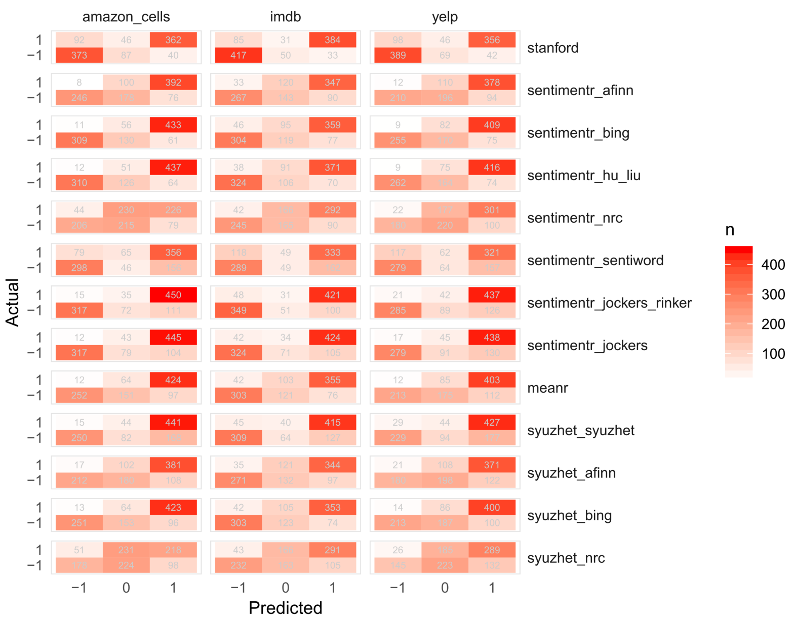
Across all three contexts, notice that the Stanford coreNLP algorithm is better at:
The Jockers, Bing, Hu & Lu, and Afinn dictionaries all do well with regard to not assigning negative scores to positive statements, but perform less well in the reverse, often assigning positive scores to negative statements, though Jockers’ dictionary outperforms the others. We can now see that the reason for the NRC’s poorer performance in accuracy rate above is its inability to discriminate. The Sentiword dictionary does well at discriminating (like Stanford’s coreNLP) but lacks accuracy. We can deduce two things from this observation:
A reworking of the Sentiword dictionary may yield better results for a dictionary lookup approach to sentiment detection, potentially, improving on discrimination and accuracy.
The reader may access the R script used to generate this visual via:
testing2 <- system.file("sentiment_testing/raw_results.R", package = "sentimentr")
file.copy(testing2, getwd())The user may wish to see the output from sentiment_by
line by line with positive/negative sentences highlighted. The
highlight function wraps a sentiment_by output
to produces a highlighted HTML file (positive = green; negative = pink).
Here we look at three random reviews from Hu and Liu’s (2004) Cannon G3
Camera Amazon product reviews.
library(magrittr)
library(dplyr)
set.seed(2)

hu_liu_cannon_reviews %>%
    filter(review_id %in% sample(unique(review_id), 3)) %>%
    mutate(review = get_sentences(text)) %$%
    sentiment_by(review, review_id) %>%
    highlight()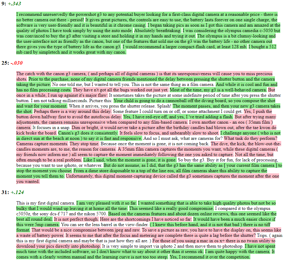
You are welcome to:
- submit suggestions and bug-reports at: https://github.com/trinker/sentimentr/issues
- send a pull request on: https://github.com/trinker/sentimentr/
- compose a friendly e-mail to:
tyler.rinker@gmail.com
These binaries (installable software) and packages are in development.
They may not be fully stable and should be used with caution. We make no claims about them.