The hardware and bandwidth for this mirror is donated by METANET, the Webhosting and Full Service-Cloud Provider.
If you wish to report a bug, or if you are interested in having us mirror your free-software or open-source project, please feel free to contact us at mirror[@]metanet.ch.
A sequencer is a device or software for creating musical pieces by editing and combining sound samples. The aim of this package is to provide a minimalistic R-based implementation of the most basic actions typically performed by a sequencer, in particular:
While this package is quite rudimentary compared with existing sequencers, it allows using the R language for automating some of these steps, which is particularly useful for data sonification, as will be illustrated in this vignette (with more examples available in this blog).
The package sequenceR strongly builds on the package
tuneR, and both packages generally need to be loaded:
library(sequenceR)
library(tuneR)A soundSample is an object containing the following
attributes:
wave, normalized to be smaller than 1 in absolute
value.duration of the sample in seconds.rate, in number of values per second.n, equal to
rate*duration.Let’s now see three possible ways to create a
soundSample object.
A 0.1-second A note can be created by using a sine wave as shown below:
# a 0.1-second A note
d <- 0.1 # duration of the sample in seconds
rate <- 44100 # sampling rate in values per second (this is a typical value and is used as a default throughout this package)
n <- round(rate*d) # number of values in the waveform
w <- sin(2*pi*440*seq(0,d,length.out=n)) # waveform (440Hz A note)
A <- soundSample(wave=w,rate=rate)
The package provides two methods to plot and
listen to the created soundSample object:
# listen(A) # uncomment to listen to the sample
plot(A) # plot the sample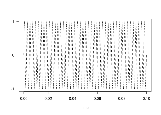
The second example below adds some noise to this perfect A note. For more approaches to generate sound, see sound synthesis.
set.seed(123456)
noisyA <- soundSample(wave=w+0.1*rnorm(n))
# listen(noisyA) # uncomment to listen to the sample
plot(noisyA)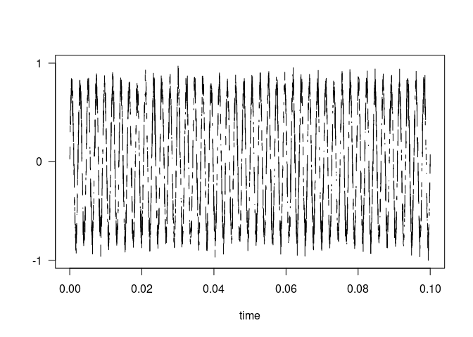
Instead of generating a sound from mathematical functions, it is possible to use an existing data series and to interpret it as a waveform as shown in the example below. This works better with relatively long series showing some form of seasonality.
sun <- soundSample(sunspots,rate=44100/10) # sampling rate is lowered to get a low pitch
# listen(sun) # uncomment to listen to the sample
plot(sun)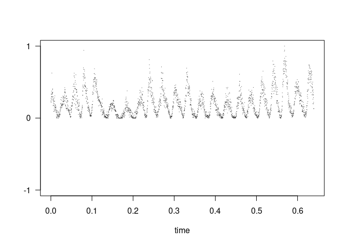
A soundSample object can also be created by reading an
existing audio file (typically a .wav or .mp3). Functions such as
readWave and readMP3 are provided by the
tuneR package for this purpose. The example below shows how
to read a ‘ding-dong’ mp3 file, downloaded from the BBC website. You
can find more sources of audio sound samples on this website.
w <- tuneR::readMP3(file.path('vignettes','07027201.mp3'))
tuneR::plot(w)
Note that the readWave function returns a
Wave object (from package tuneR), which needs
to be turned into a soundSample object (from package
sequenceR). This can easily be done as shown below.
Comparing the plots above and below illustrates the main differences
between Wave and soundSample objects: (1) the
latter is mono, while the former may be stereo; (2) the latter is
standardized so that its maximum absolute value is one.
# Cast Wave to sound Sample
sam <-as.soundSample(w)
# listen(sam) # uncomment to listen to the sample
plot(sam)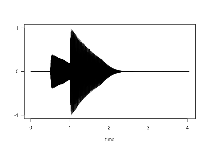
The sequence function repeats a soundSample
at specific times (given in seconds). It is also possible to specify the
volume (standardized between 0 and 1) at which each repetition is
played, along with its panoramic (-1 for full left to 1 for full right,
0 is centered). The example below illustrates this. Note that the output
of the sequence function is a stereo Wave
object.
A_seq <- sequence(A,time=c(0,0.5,1,1.5),
                  volume=c(1,0.4,0.4,0.4),
                  pan=c(0,-0.5,0.5,1))
tuneR::plot(A_seq)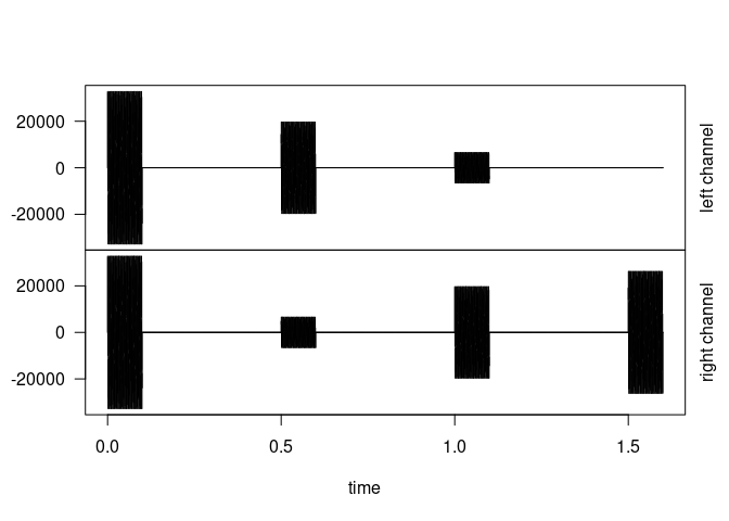
The code below creates a second sequence using the sample read from
the BBC website, and illustrate the effect of the option
letRing.
sam_seq <- sequence(sam,time=c(0,1.2),pan=c(-1,1),letRing=FALSE)
tuneR::plot(sam_seq)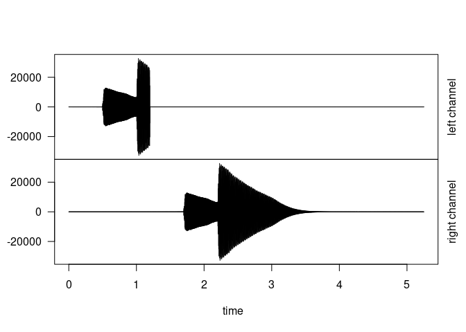
sam_seq <- sequence(sam,time=c(0,1.2),pan=c(-1,1),letRing=TRUE)
tuneR::plot(sam_seq)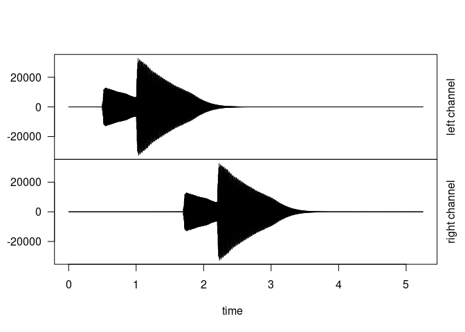
The mix function takes several Wave objects
as inputs (e.g. sequences resulting from calls to the
sequence function) and merges them into a single
Wave object. It allows controlling the volume and the
panoramic of each sequence.
myMix <- mix(list(A_seq,sam_seq),volume=c(1,0.3))
# tuneR::play(myMix) # uncomment to play
# tuneR::writeWave(myMix,'myMix.wav') # uncomment to save to disk
tuneR::plot(myMix)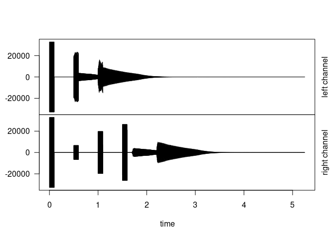
Data sonification refers to the transformation of data into sound, using some algorithmic process. This can be achieved in many ways, but here we focus on the approach known as parameter mapping: the values taken by the data are mapped into some attributes (or parameters) of notes, typically their pitch or loudness, or possibly their duration. This is very much the same process as the mapping performed in data visualization, where data values are mapped into e.g. the color, size of type of symbols in a graph or map.
One possible sonification process is to use data to control the
sequencing of a sound sample. Consider, as an example, the Wagga Wagga
dataset which comes with this package. It contains the annual
precipitation and temperature time series in the city of Wagga Wagga,
New South Wales, Australia, as plotted below. A possible sonification of
this dataset is to use the data to control the elements of a drum. For
instance, a low kick might be played whenever the precipitation is low,
and a snare whenever it is high; in addition the temperature might be
used to control the master volume. The use of sequenceR to
achieve this is described next.
plot(WaggaWagga$Year,WaggaWagga$Precipitation,type='l',xlab='Year',ylab='precip. [mm]')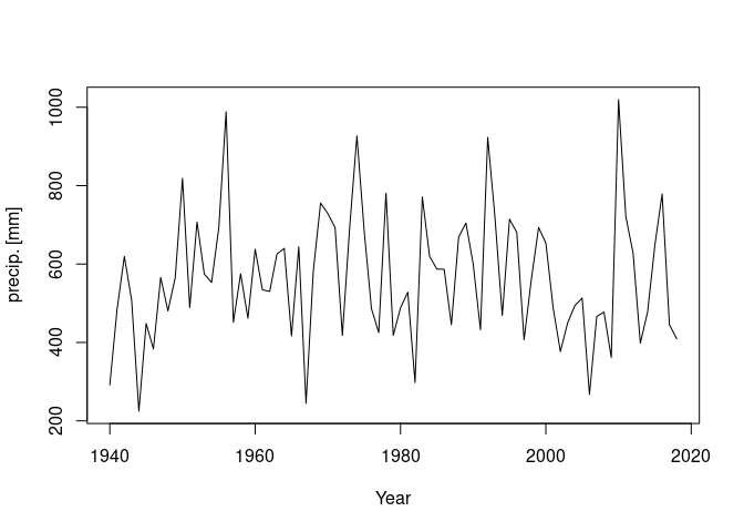
plot(WaggaWagga$Year,WaggaWagga$Temperature,type='l',xlab='Year',ylab='temp. [C]')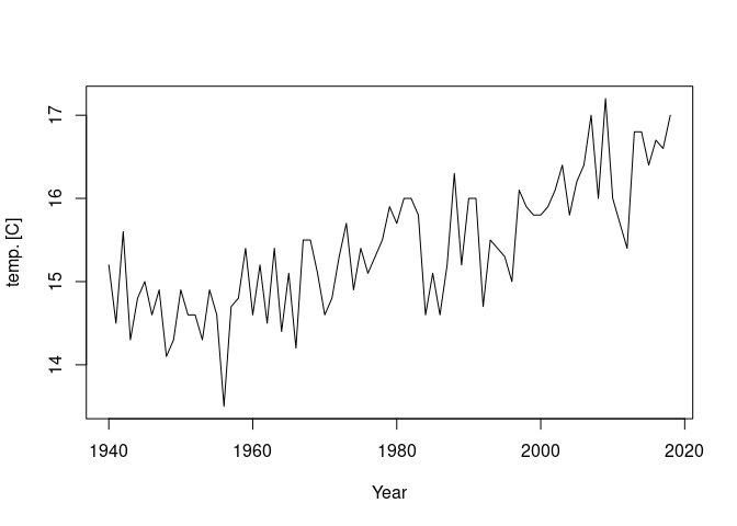
We start by defining a few properties of this sonification attempt: its duration, the times at which sound samples will be played and the master volume, controlled by the temperature time series.
n <- NROW(WaggaWagga) # series size
dur <- 9 # duration in seconds
tim <- dur*seq(0,1,length.out=n) # regular time vector between 0 and dur
master <- rescale(WaggaWagga$Temperature,0.2,1) # master volume = temperature time series rescaled between 0.2 and 1
We are going to use three basic elements of a drum: a hi-hat, a bass
drum and a snare. The corresponding soundSample objects
hiHat, kick and snare come along
with this package so that we can directly proceed to the sequencing.
We start by defining a hi-hat rhythmic pattern by playing groups of four notes, the first one being accentuated. This is a typical pattern (very much similar to this intro) and it allows installing the rhythmic pulse.
every4=(((1:n)-1))%%4==0 # T F F F T F F F etc.
accents <- rescale(as.numeric(every4),0.2,1) # 1 0.2 0.2 0.2 1 0.2 0.2 0.2 etc.
hh <- sequence(hiHat,time=tim,volume=master*accents) # create hi-hat sequence
# tuneR::play(hh) # uncomment to play
We then define the low kick sequence by playing it every time precipitation is lower than some threshold.
mask=WaggaWagga$Precipitation<450 # time steps with low pp
k <- sequence(kick,time=tim[mask],volume=master[mask]) # play a kick at those time steps
# tuneR::play(k) # uncomment to play
We proceed in a similar way to associate the snare with high precipitation values.
mask=WaggaWagga$Precipitation>800 # time steps with high pp
s <- sequence(snare,time=tim[mask],volume=master[mask]) # play a snare at those time steps
# tuneR::play(s) # uncomment to play
The final step is to mix the hi-hat, kick and snare sequences together and to save the result to a file.
final <- mix(list(hh,k,s),volume=c(0.5,0.75,1))
writeWave(final,'WaggaWagga.wav') # write to disc
# tuneR::play(final) # uncomment to play
Data sonification is particularly interesting when it is combined with data animation, as shown in the example below based on the package gganimate. The resulting video can be seen here.
library(tidyr);library(ggplot2);library(gganimate)
# Modify the shape of the WaggaWagga dataset to facilitate plotting
DF <- pivot_longer(WaggaWagga,-Year) # function from tidyr
# Plot precipitation and temperature time series using ggplot
g <- ggplot(DF,aes(x=Year,y=value))
g <- g + geom_line(aes(color=name),linewidth=1)+geom_point(size=4)
g <- g + scale_color_manual(values = c('blue','red'),guide=FALSE)
g <- g + facet_wrap(vars(name),ncol=1,scales='free_y')+theme_bw()
g <- g + geom_hline(data=data.frame(y=450,name='Precipitation'),aes(yintercept=y))
g <- g + geom_hline(data=data.frame(y=800,name='Precipitation'),aes(yintercept=y))
# Make it look nicer
g <- g+theme_bw()+theme(axis.title=element_text(size=18),
          axis.text=element_text(size=14),
          strip.text=element_text(size=18))
# Create an animated plot
g <- g + transition_reveal(Year)
# 'Render' the animated plot into a .mp4 movie
fps=n/dur # number of frames divided by duration
animate(g,nframes=NROW(WaggaWagga),fps=fps,width=1280,height=720,
renderer = av_renderer('WaggaWaggaGroove.mp4',audio='WaggaWagga.wav'))An instrument object is simply a named list of
soundSample’s. For instance, a simple drum kit can be
assembled using the kick, snare and
hiHat soundSample’s that come with the
package. The instrument can then be played using the
play.instrument function, which is mostly an extension of
the sequence function to allow selecting notes:
drums <- instrument(samples=list(kick,snare,hiHat),notes=c('boom','tat','cheet'))
w=play.instrument(drums,notes=rep(c('boom','cheet','tat','cheet'),4),
                  time=0.25*(0:15),volume=(1:16)/16,
                  pan=rep(c(0,-0.5,0.5,-0.5),4))
# tuneR::play(w) # uncomment to play
tuneR::plot(w)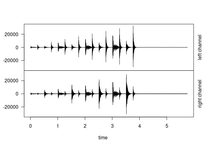
Instruments are very useful to implement data sonification: many examples can be found in this blog (with corresponding codes here). It is possible to build your own instruments using the many sample packs that can be downloaded from the internet (not for free in general). On this page you will find several links to freely-available packs, generally under an “attribution” creative commons license. This file can be used to build the instrument from downloaded packs.
The package provides a few basic tools for sound synthesis:
oscillator utilities (see ?oscillator and
?oscillator_pattern) and a basic synthesizer:
# Create a synthesizer instrument and play it
synth <- getSynth(c('E2','B2','E3','G3','A3'))
w=play.instrument(synth,time=(0:(length(synth)-1))*0.5,fadeout=rep(Inf,length(synth)))
# tuneR::play(w) # uncomment to play
tuneR::plot(w)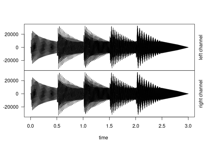
The package provides a few basic effects: envelopes, distortion and delay:
dry=oscillator(freq=110,duration=1) # a low A note
# Define an ADSR envelope (https://en.wikipedia.org/wiki/Envelope_(music)#ADSR)
env <- envelope(t=c(0,0.05,0.2,0.8,1),v=c(0,1,0.6,0.2,0))
plot(env)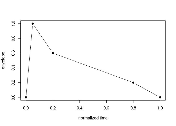
# Apply effects: envelope, saturation and delay
w1=applyEnvelope(dry,env)
w2=applyDisto(w1,type='clip',level=0.5)
wet=applyDelay(w2,delayTime=0.5,echoes=1/(1:5))
# listen(wet) # uncomment to play
plot(wet)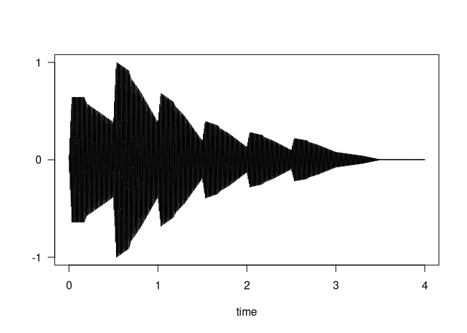
The piping syntax of dplyr is quite useful for chaining
effects:
library(dplyr)
wet=dry %>% applyEnvelope(env) %>% applyDisto(type='clip',level=0.5) %>%
  applyDelay(delayTime=0.5,echoes=1/(1:5))
# listen(wet) # uncomment to play
plot(wet)
The package provides a pre-built sonification of the famous warming stripes: this allows using your own data, playing with musical options, and digging into the code to see how the tools provided by the package can be pieced together to create music out of data.
w=sonifyStripes(videoFile='stripes.mp4')These binaries (installable software) and packages are in development.
They may not be fully stable and should be used with caution. We make no claims about them.