The hardware and bandwidth for this mirror is donated by METANET, the Webhosting and Full Service-Cloud Provider.
If you wish to report a bug, or if you are interested in having us mirror your free-software or open-source project, please feel free to contact us at mirror[@]metanet.ch.

shewhartr

shewhartr is a tidyverse-native toolkit for Statistical Process Control (SPC). It implements the classical Shewhart chart family — variables (I-MR, Xbar-R, Xbar-S) and attributes (p, np, c, u) — alongside a flagship regression-based control chart for processes with trend, where stationarity is too strong an assumption to make.

The package is built around a small set of design choices:

• Tidy by default. Every constructor takes data first, supports tidy-eval column references, and returns an S3 object that integrates with broom via tidy(), glance() and augment().
• Diagnostics in the box. Average Run Length (ARL) by Monte Carlo simulation, all eight Nelson runs rules, Box-Cox guidance, and a Tukey-style residual panel are first-class citizens.
• Phase I / Phase II. Explicit calibrate() and monitor() functions make the distinction between estimation and prospective monitoring impossible to confuse, following Woodall (2000).
• Multilingual plots. Pass locale = "pt" (or "es", "fr") and chart titles, axis labels, and legends are translated.
• Statistically honest counts. c and u charts accept limits = "poisson" for exact Poisson quantile limits, instead of the normal approximation that breaks down at small means.

Installation

# Development version
remotes::install_github("castlaboratory/shewhartr")

A 30-second tour

library(shewhartr)
library(ggplot2)

# Classical I-MR chart on a 100-observation series with a small drift
fit <- shewhart_i_mr(bottle_fill, value = ml, index = observation)

print(fit)
autoplot(fit)

When to use which chart

Multi-phase regression chart

The flagship chart for trended processes splits the series into phases when a runs rule fires, fits a local model in each, and flags points that depart from the local trend. The example below uses the COVID-19 mortality series for Recife (cvd_recife) with the original analysis settings from Ferraz et al. (2020):

fit <- shewhart_regression(
  cvd_recife,
  value       = new_deaths,
  index       = .t,
  model       = "loglog",
  phase_rule  = "we_seven_same",
  rules       = c("nelson_1_beyond_3s", "we_seven_same"),
  lower_bound = 0
)

length(fit$fits)              # number of phases detected
nrow(fit$violations)          # individual flagged observations
autoplot(fit)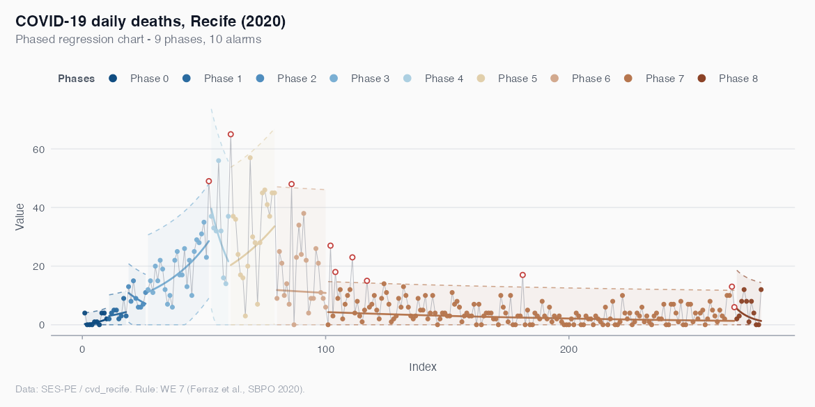

Each shaded band is one phase, the solid line is the local regression centre, the dashed lines are the phase’s 3-sigma limits, and the firebrick points are the days flagged by the rule set as departing from the local trend.

Phase I vs Phase II

A Shewhart chart serves two different purposes that are easy to conflate. Phase I is retrospective: take historical data, identify out-of-control points, eliminate assignable causes, and arrive at trustworthy estimates of the process mean and variability. Phase II is prospective: take those estimated limits and apply them to new data, signalling alarms when something departs from the established baseline. The package draws this line in code:

# Phase I: estimate limits from a clean baseline
calib <- calibrate(historical_data, value = y,
                   chart = "i_mr", trim_outliers = TRUE)

# Phase II: apply the limits to new data
alarms <- monitor(new_observations, calib)
alarms$violations

Architecture

Every chart constructor — variables (shewhart_i_mr, shewhart_xbar_r, shewhart_xbar_s), attributes (shewhart_p, shewhart_np, shewhart_c, shewhart_u), regression (shewhart_regression), memory-based (shewhart_ewma, shewhart_cusum), and multivariate (shewhart_hotelling) — returns a shewhart_chart S3 object with a uniform layout. The same object then feeds into:

• Inspect: print(), summary(), shewhart_diagnostics(), shewhart_capability(), shewhart_arl().
• Plot: autoplot() (ggplot2) and as_plotly() (interactive, plotly in Suggests).
• Tidy: broom::tidy(), glance(), augment().
• Phase II: calibrate() produces a Phase I chart whose limits are frozen by monitor() for prospective monitoring.

Documentation

The website hosts:

• A full reference for every exported function.
• Topical articles: variables charts, attributes charts, regression charts, Phase I/II, ARL by simulation, residual diagnostics, Box-Cox guidance.
• A case study on epidemiological monitoring with the regression chart.

Citation

If you use shewhartr in academic work, please cite:

Leite, A., Vasconcelos, H., Ospina, R., & Ferraz, C. (2025). shewhartr: Statistical Process Control with Tidyverse-Native Workflows. R package version 1.0.0. https://castlaboratory.github.io/shewhartr/

References

• Shewhart, W. A. (1931). Economic Control of Quality of Manufactured Product. D. Van Nostrand.
• Montgomery, D. C. (2019). Introduction to Statistical Quality Control (8th ed.). Wiley.
• Nelson, L. S. (1984). The Shewhart Control Chart — Tests for Special Causes. Journal of Quality Technology, 16(4), 237-239.
• Woodall, W. H. (2000). Controversies and Contradictions in Statistical Process Control. Journal of Quality Technology, 32(4), 341-350.
• Box, G. E. P., & Cox, D. R. (1964). An Analysis of Transformations. Journal of the Royal Statistical Society B, 26(2), 211-252.
• Tukey, J. W. (1977). Exploratory Data Analysis. Addison-Wesley.
• Wheeler, D. J., & Chambers, D. S. (1992). Understanding Statistical Process Control (2nd ed.). SPC Press.
• Perla, R. J., Provost, S. M., Parry, G. J., Little, K., & Provost, L. (2020). Understanding variation in reported COVID-19 deaths with a novel Shewhart chart application. International Journal for Quality in Health Care, 32(S1), 49-55.
• Ferraz, C., Petenate, A. J., Wanderley, A. L., Ospina, R., Torres, J., & Moreira, A. P. (2020). COVID-19: Monitoramento por gráficos de Shewhart. Revista Brasileira de Estatística.

These binaries (installable software) and packages are in development.
They may not be fully stable and should be used with caution. We make no claims about them.