The hardware and bandwidth for this mirror is donated by METANET, the Webhosting and Full Service-Cloud Provider.
If you wish to report a bug, or if you are interested in having us mirror your free-software or open-source project, please feel free to contact us at mirror[@]metanet.ch.

slasso

The package slasso implements the smooth LASSO estimator (S-LASSO) for the Function-on-Function linear regression model proposed by Centofanti et al. (2020). The S-LASSO estimator is able to increase the interpretability of the model, by better locating regions where the coefficient function is zero, and to smoothly estimate non-zero values of the coefficient function. The sparsity of the estimator is ensured by a functional LASSO penalty, which pointwise shrinks toward zero the coefficient function, while the smoothness is provided by two roughness penalties that penalize the curvature of the final estimator. The package comprises two main functions slasso.fr and slasso.fr_cv. The former implements the S-LASSO estimator for fixed tuning parameters of the smoothness penalties λ_s and λ_t, and tuning parameter of the functional LASSO penalty λ_L. The latter executes the K-fold cross-validation procedure described in Centofanti et al. (2020) to choose λ_L, λ_s, and λ_t.

Installation

The development version can be installed from GitHub with:

# install.packages("devtools")
devtools::install_github("unina-sfere/slasso")

Example

This is a basic example which shows you how to apply the two main functions slasso.fr and slasso.fr_cv on a synthetic dataset generated as described in the simulation study of Centofanti et al. (2020).

We start by loading and attaching the slasso package.

library(slasso)

Then, we generate the synthetic dataset and build the basis function sets as follows.

data<-simulate_data("Scenario II",n_obs=500)
X_fd=data$X_fd
Y_fd=data$Y_fd
domain=c(0,1)
n_basis_s<-30
n_basis_t<-30
breaks_s<-seq(0,1,length.out = (n_basis_s-2))
breaks_t<-seq(0,1,length.out = (n_basis_t-2))
basis_s <- fda::create.bspline.basis(domain,breaks=breaks_s)
basis_t <- fda::create.bspline.basis(domain,breaks=breaks_t)

To apply slasso.fr_cv, sequences of λ_L, λ_s, and λ_t should be defined.

lambda_L_vec=10^seq(0,1,by=0.1) 
lambda_s_vec=10^seq(-6,-5) 
lambda_t_vec=10^seq(-5,-5) 

And, then, slasso.fr_cv is executed.

mod_slasso_cv<-slasso.fr_cv(Y_fd = Y_fd,X_fd=X_fd,basis_s=basis_s,basis_t=basis_t,
lambda_L_vec = lambda_L_vec,lambda_s_vec = lambda_s_vec,lambda_t_vec =lambda_t_vec,
max_iterations=1000,K=10,invisible=1,ncores=12)

The results are plotted.

plot(mod_slasso_cv)

By using the model selection method described in Centofanti et al. (2020), the optimal values of λ_L, λ_s, and λ_t, are 3.98, 10^− 5, and 10^− 5, respectively.

Finally, sasfclust is applied with λ_L, λ_s, and λ_t fixed to their optimal values.

mod_slasso<-slasso.fr(Y_fd = Y_fd,X_fd=X_fd,basis_s=basis_s,basis_t=basis_t,
lambda_L = mod_slasso_cv$lambda_opt_vec[1],lambda_s = mod_slasso_cv$lambda_opt_vec[2],
lambda_t =  mod_slasso_cv$lambda_opt_vec[3],invisible=1,max_iterations=1000)

The resulting estimator is plotted as follows.

plot(mod_slasso)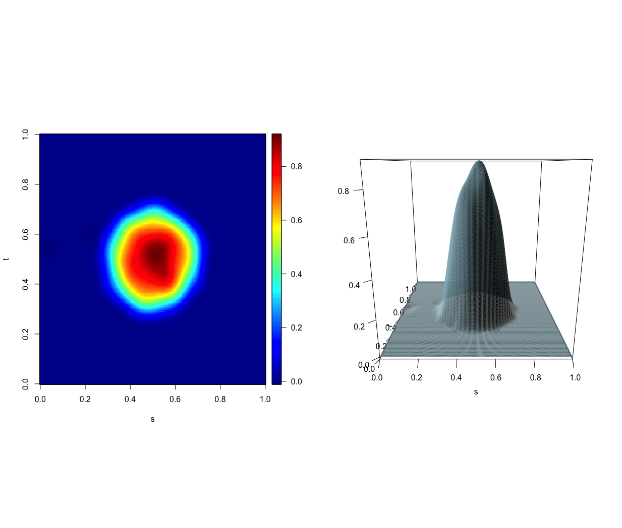

References

• Centofanti, F., Fontana, M., Lepore, A., & Vantini, S. (2020). Smooth LASSO Estimator for the Function-on-Function Linear Regression Model. arXiv preprint arXiv:2007.00529.

These binaries (installable software) and packages are in development.
They may not be fully stable and should be used with caution. We make no claims about them.