The hardware and bandwidth for this mirror is donated by METANET, the Webhosting and Full Service-Cloud Provider.
If you wish to report a bug, or if you are interested in having us mirror your free-software or open-source project, please feel free to contact us at mirror[@]metanet.ch.

snapKrig

An R package for fast spatial analysis and kriging on grids

snapKrig uses a computationally lean implementation of a 2-dimensional spatial correlation model for gridded data. By restricting to models with (separable) Kronecker covariance, the package can speed computations on certain likelihood and kriging problems by orders of magnitude compared to alternatives like gstat, fields, geoR, spatial, and LatticeKrig.

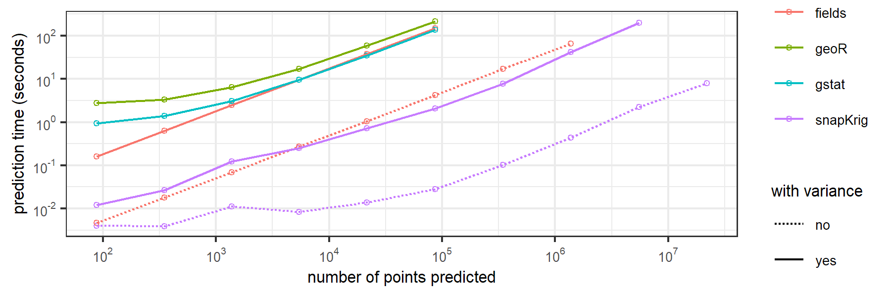
Here are some benchmarking results for computation time to downscale a 32 x 43 raster onto grids of increasing size by ordinary kriging.

code and instructions to reproduce these results can be found here

Installation

snapKrig is on CRAN. Install it with

install.packages('snapKrig')

or use devtools to install the latest development version

devtools::install_github('deankoch/snapKrig')

Check out the introduction vignette for a worked example with the Meuse soils data, or try the code below to get started right away. Some other code examples be found here. We plan to publish a more detailed tutorial and benchmarking study in an upcoming paper.

Example

To get started define an empty grid

library(snapKrig)

# simulate data on a rectangular grid
g_empty = sk(c(100, 200))
g_empty
#> 100 x 200 empty

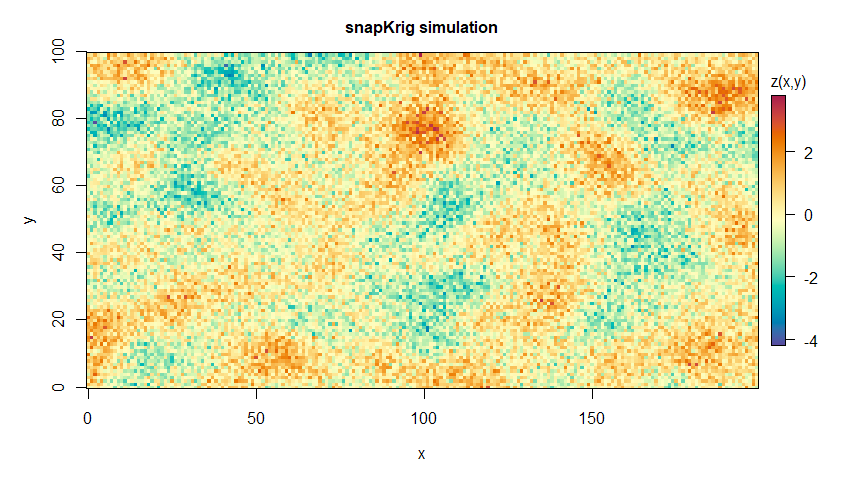
Generate some random auto-correlated data for this grid

# set a random seed
set.seed(1234567)

# simulate data on a square grid
pars = sk_pars(g_empty)
g_sim = sk_sim(g_empty, pars)

# plot
plot(g_sim, main='snapKrig simulation')

g_sim
#> 100 x 200 complete

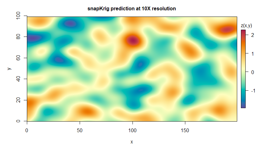
Downscale and filter noise by simple kriging

# downscale and predict, timing computations
t_start = Sys.time()
g_down = sk_rescale(g_sim, down=10)
g_pred = sk_cmean(g_down, pars, X=0)
#> 100 x 200 complete sub-grid detected

# print time elapsed in computation
t_end = Sys.time()
t_end - t_start
#> Time difference of 0.7008011 secs

# plot grid
plot(g_pred, main='snapKrig prediction at 10X resolution')

# print summary
summary(g_pred)
#> complete sk grid
#> 1973081 points
#> range [-1.95, 2.26]
#> ..............................
#> dimensions : 991 x 1991
#> resolution : 0.1 x 0.1
#>     extent : [0, 99] x [0, 199]

Technical Features

snapKrig’s computational efficiency makes it useful in situations where interpolation or down-scaling would pose a problem due to long computation times and/or high memory demands. Such problems are common when working with geo-referenced data in earth sciences. snapKrig’s features include:

• anisotropic Gaussian processes on 2-dimensional regular grids for a choice of covariance kernels
• optimized computation of the likelihood function, generalized least squares, and kriging predictor/variance
• fast computations with missing data problems, and even faster in the complete data case
• automated maximum likelihood model fitting and support for sample semi-variograms
• user friendly helper functions for raster down-scaling and point interpolation

snapKrig depends only on packages included by default in R (like graphics and stats), but supports raster and geometry classes from sf and terra.

History

An earlier implementation of snapKrig was called pkern. snapKrig is a redesigned version that uses a more user-friendly S3 grid object class.

pkern was an R implementation of some methods I developed in my thesis for speeding up geostatistical computations involving large covariance matrices. The central idea is to model spatial dependence using a separable 2-dimensional covariance kernel, defined as the product of two (1-dimensional) univariate covariance kernels. This introduces special symmetries and structure in the covariance matrix, which are exploited in this package for fast and memory-efficient computations.

I developed snapKrig to support a project to interpolate weather data, but the methods underlying snapKrig are applicable more generally. See also [1], where I use product kernels to study directions of anisotropy in a non-stationary random fields, and [2, 3], where I apply it to fit a covariance structure, and to speed up calculations of dispersal kernel convolutions.

These binaries (installable software) and packages are in development.
They may not be fully stable and should be used with caution. We make no claims about them.