The hardware and bandwidth for this mirror is donated by METANET, the Webhosting and Full Service-Cloud Provider.
If you wish to report a bug, or if you are interested in having us mirror your free-software or open-source project, please feel free to contact us at mirror[@]metanet.ch.

snvecR

Easily calculate precession and obliquity from an astronomical solution (AS, defaults to ZB18a from Zeebe and Lourens (2019)) and assumed or reconstructed values for tidal dissipation (T_d) and dynamical ellipticity (E_d). This is a translation and adaptation of the C-code in the supplementary material to Zeebe and Lourens (2022), with further details on the methodology described in Zeebe (2022). The name of the C-routine is snvec, which refers to the key units of computation: spin vector s and orbit normal vector n.

Installation

You can install snvecR like so:

install.packages("snvecR")

To use the development version of the package, use:

remotes::install_github("japhir/snvecR")

Example

Here’s the main function that does the work in action:

library(snvecR)
solution <- snvec(tend = -1000, # final timestep in kyr
                  ed = 1, # dynamical ellipticity, normalized to modern
                  td = 0, # tidal dissipation, normalized to modern
                  astronomical_solution = "full-ZB18a", # see ?full_ZB18a for details
                  tres = -0.4 # timestep resolution in kyr (so this is 400 years)
                  )
#> ℹ The astronomical solution "full-ZB18a" has not been downloaded.
#> ℹ Reading 'full-ZB18a.dat' from website <http://www.soest.hawaii.edu/oceanography/faculty/zeebe_files/Astro/PrecTilt/OS/ZB18a/ems-plan3.dat>.
#> ℹ Calculating helper columns.
#> ℹ The cache directory is '/home/japhir/.cache/R/snvecR'.
#> ℹ Saved 'full-ZB18a.dat' to cache.
#> ℹ Saved cleaned-up 'full-ZB18a.csv' to cache.
#> ℹ Saved astronomical solution with helper columns 'full-ZB18a.rds' to cache.
#> ℹ Future calls to `get_solution("full-ZB18a")` will read from the cache.
#> ! If you don't want this, specify `force = TRUE`.
#> This is snvecR VERSION: 3.9.2.9000 2024-04-22
#> Richard E. Zeebe
#> Ilja J. Kocken
#> 
#> Integration parameters:
#> • `tend` = -1000 kyr
#> • `ed` = 1
#> • `td` = 0
#> • `astronomical_solution` = "full-ZB18a"
#> • `os_ref_frame` = "HCI"
#> • `os_omt` = defaulting to 75.594
#> • `os_inct` = defaulting to 7.155
#> • `tres` = -0.4 kyr
#> • `atol` = 1e-05
#> • `rtol` = 0
#> • `solver` = "vode"
#> ℹ started at "2024-04-22 08:47:29.732434"
#> Final values:
#> • s[1][2][3]: 0.404184487124565, -0.0537555129057148, and 0.913036138471423
#> • s-error = |s|-1: -5.51290422495798e-05
#> Final values:
#> • obliquity: 0.413060472710089 rad
#> • precession: -0.562357122261026 rad
#> ℹ stopped at "2024-04-22 08:47:34.762126"
#> ℹ total duration: 5.03

To quickly save out the results for further study to CSV¹:

write.csv(solution, "ZB18a_ed-1.0_td-0.0.csv")

see ?snvec for further documentation.

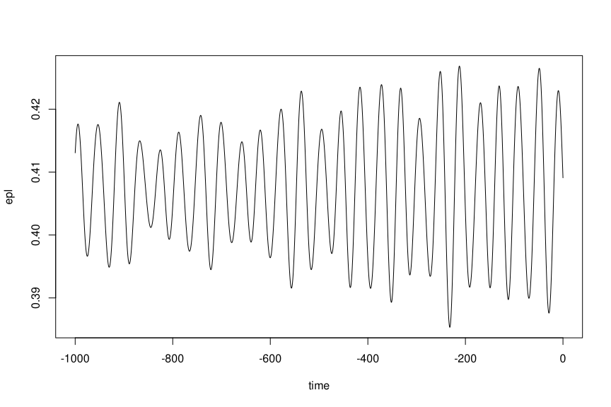
Here we create a quick plot of the obliquity:

plot(epl ~ time, data = solution, type = 'l')

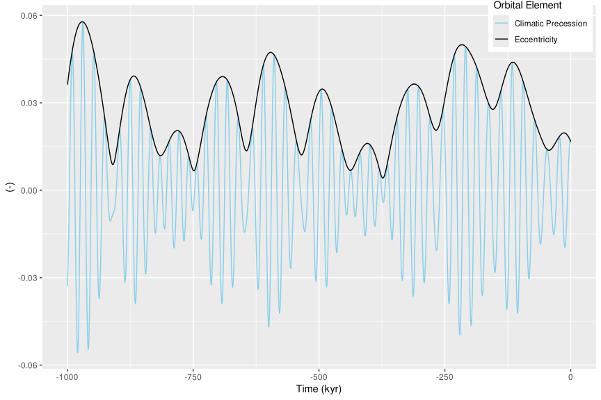
Or if you want to make a slightly fancier plot of the calculated climatic precession with the eccentricity envelope:

library(ggplot2)
solution |>
  ggplot(aes(x = time, y = cp)) +
  labs(x = "Time (kyr)", y = "(-)", colour = "Orbital Element") +
  # plot climatic precession
  geom_line(aes(colour = "Climatic Precession")) +
  # add the eccentricity envelope
  geom_line(aes(y = ee, colour = "Eccentricity"),
            data = get_solution() |> dplyr::filter(time > -1000)) +
  scale_color_discrete(type = c("skyblue", "black")) +
  theme(legend.position = "inside", legend.position.inside = c(.9, .95))

References

Zeebe, R. E., & Lourens, L. J. (2019). Solar System chaos and the Paleocene–Eocene boundary age constrained by geology and astronomy. Science, 365(6456), 926–929. doi:10.1126/science.aax0612.

Zeebe, R. E., & Lourens, L. J. (2022). A deep-time dating tool for paleo-applications utilizing obliquity and precession cycles: The role of dynamical ellipticity and tidal dissipation. Paleoceanography and Paleoclimatology, e2021PA004349. doi:10.1029/2021PA004349.

Zeebe, R. E. (2022). Reduced Variations in Earth’s and Mars’ Orbital Inclination and Earth’s Obliquity from 58 to 48 Myr ago due to Solar System Chaos. The Astronomical Journal, 164(3), doi:10.3847/1538-3881/ac80f8.

Wikipedia page on Orbital Elements: https://en.wikipedia.org/wiki/Orbital_elements

These binaries (installable software) and packages are in development.
They may not be fully stable and should be used with caution. We make no claims about them.