The hardware and bandwidth for this mirror is donated by METANET, the Webhosting and Full Service-Cloud Provider.
If you wish to report a bug, or if you are interested in having us mirror your free-software or open-source project, please feel free to contact us at mirror[@]metanet.ch.
![]()
![]()
![]()
The goal of spatialising is to perform simulations of binary spatial raster data using the Ising model.
You can install the released version of spatialising from CRAN with:
install.packages("spatialising")You can install the development version of spatialising from GitHub with:
# install.packages("devtools")
devtools::install_github("Nowosad/spatialising")The spatialising package expects raster data with
just two values, -1 and 1. Here, we will use
the r_start.tif file built in the package.
library(spatialising)
library(terra)
r1 = rast(system.file("raster/r_start.tif", package = "spatialising"))
plot(r1)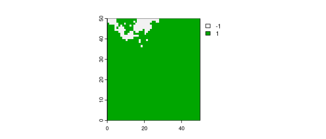
Most of the raster area is covered with the value of 1,
and just about 5% of the area is covered with the value of
-1. The main function in this package is
kinetic_ising(). It accepts the input raster and at least
two additional parameters: B – representing external
pressure and J – representing the strength of the local
autocorrelation tendency. The output is a raster modified based on the
provided parameters.
r2 = kinetic_ising(r1, B = -0.3, J = 0.7)
plot(r2)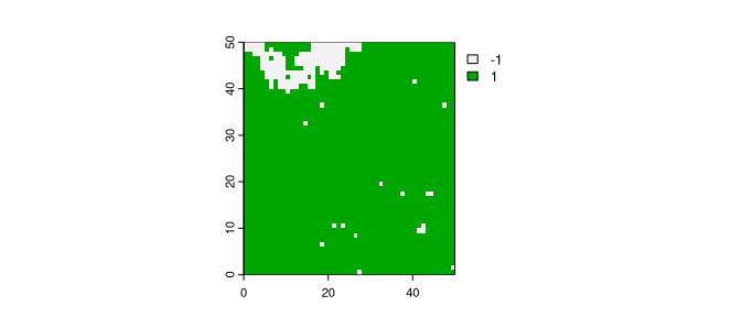
The kinetic_ising() function also has a fourth argument
called updates. By default, it equals to 1,
returning just one raster as the output. However, when given a value
larger than one, it returns many rasters. Each new raster is the next
iteration of the Ising model of the previous one.
ri1 = kinetic_ising(r1, B = -0.3, J = 0.7, updates = 3)
plot(ri1, nr = 1)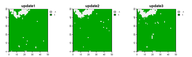
Obtained results depend greatly on the set values of B
and J. In the example above, values of
B = -0.3 and J = 0.7 resulted in expansion of
the yellow category (more -1 values).
On the other hand, values of B = 0.3 and
J = 0.7 give a somewhat opposite result with less cell with
the yellow category:
ri2 = kinetic_ising(r1, B = 0.3, J = 0.7, updates = 3)
plot(ri2, nr = 1)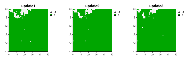
Finally, in the last example, we set values of B = -0.3
and J = 0.4. Note that the result shows much more prominent
data change, with a predominance of the yellow category only after a few
updates.
ri3 = kinetic_ising(r1, B = -0.3, J = 0.4, updates = 3)
plot(ri3, nr = 1)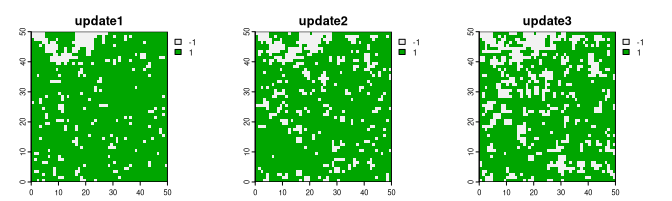
Read the related article:
Contributions to this package are welcome - let us know if you have any suggestions or spotted a bug. The preferred method of contribution is through a GitHub pull request. Feel also free to contact us by creating an issue.
These binaries (installable software) and packages are in development.
They may not be fully stable and should be used with caution. We make no claims about them.