The hardware and bandwidth for this mirror is donated by METANET, the Webhosting and Full Service-Cloud Provider.
If you wish to report a bug, or if you are interested in having us mirror your free-software or open-source project, please feel free to contact us at mirror[@]metanet.ch.
survalis provides a unified framework for survival
machine learning survival analysis in R. It supports a wide range of
learners, evaluation metrics, cross-validation and interpretability
methods.
# Install from GitHub
remotes::install_github("ielbadisy/survalis")

# Or from source
install.packages("survalis_0.7.0.tar.gz", repos = NULL, type = "source")fit_*(),
predict_*(), tune_*()mlsurv_model objectsdata.frame of survival
probabilities: t=100, t=200, …fit_*/predict_* with
cv_survlearner() or score_survmodel()library(survalis)
# See all available learners
list_survlearners()
#> # A tibble: 19 × 8
#> learner fit predict tune has_fit has_predict has_tune available
#> <chr> <chr> <chr> <chr> <lgl> <lgl> <lgl> <lgl>
#> 1 coxph fit_cox… predic… <NA> TRUE TRUE FALSE TRUE
#> 2 aalen fit_aal… predic… <NA> TRUE TRUE FALSE TRUE
#> 3 glmnet fit_glm… predic… tune… TRUE TRUE TRUE TRUE
#> 4 selectcox fit_sel… predic… tune… TRUE TRUE TRUE TRUE
#> 5 aftgee fit_aft… predic… <NA> TRUE TRUE FALSE TRUE
#> 6 flexsurvreg fit_fle… predic… tune… TRUE TRUE TRUE TRUE
#> 7 stpm2 fit_stp… predic… <NA> TRUE TRUE FALSE TRUE
#> 8 bnnsurv fit_bnn… predic… tune… TRUE TRUE TRUE TRUE
#> 9 rpart fit_rpa… predic… tune… TRUE TRUE TRUE TRUE
#> 10 bart fit_bart predic… tune… TRUE TRUE TRUE TRUE
#> 11 xgboost fit_xgb… predic… tune… TRUE TRUE TRUE TRUE
#> 12 ranger fit_ran… predic… tune… TRUE TRUE TRUE TRUE
#> 13 rsf fit_rsf predic… tune… TRUE TRUE TRUE TRUE
#> 14 cforest fit_cfo… predic… tune… TRUE TRUE TRUE TRUE
#> 15 blackboost fit_bla… predic… tune… TRUE TRUE TRUE TRUE
#> 16 survsvm fit_sur… predic… tune… TRUE TRUE TRUE TRUE
#> 17 survdnn fit_sur… predic… tune… TRUE TRUE TRUE TRUE
#> 18 orsf fit_orsf predic… tune… TRUE TRUE TRUE TRUE
#> 19 survmetalearner fit_sur… predic… <NA> TRUE TRUE FALSE TRUE
# See only tunable learners (those with a tune_* function)
list_survlearners(has_tune = TRUE)
#> # A tibble: 14 × 8
#> learner fit predict tune has_fit has_predict has_tune available
#> <chr> <chr> <chr> <chr> <lgl> <lgl> <lgl> <lgl>
#> 1 glmnet fit_glmnet predic… tune… TRUE TRUE TRUE TRUE
#> 2 selectcox fit_selectc… predic… tune… TRUE TRUE TRUE TRUE
#> 3 flexsurvreg fit_flexsur… predic… tune… TRUE TRUE TRUE TRUE
#> 4 bnnsurv fit_bnnsurv predic… tune… TRUE TRUE TRUE TRUE
#> 5 rpart fit_rpart predic… tune… TRUE TRUE TRUE TRUE
#> 6 bart fit_bart predic… tune… TRUE TRUE TRUE TRUE
#> 7 xgboost fit_xgboost predic… tune… TRUE TRUE TRUE TRUE
#> 8 ranger fit_ranger predic… tune… TRUE TRUE TRUE TRUE
#> 9 rsf fit_rsf predic… tune… TRUE TRUE TRUE TRUE
#> 10 cforest fit_cforest predic… tune… TRUE TRUE TRUE TRUE
#> 11 blackboost fit_blackbo… predic… tune… TRUE TRUE TRUE TRUE
#> 12 survsvm fit_survsvm predic… tune… TRUE TRUE TRUE TRUE
#> 13 survdnn fit_survdnn predic… tune… TRUE TRUE TRUE TRUE
#> 14 orsf fit_orsf predic… tune… TRUE TRUE TRUE TRUE
# Shortcut for tunable learners
list_tunable_survlearners()
#> # A tibble: 14 × 8
#> learner fit predict tune has_fit has_predict has_tune available
#> <chr> <chr> <chr> <chr> <lgl> <lgl> <lgl> <lgl>
#> 1 glmnet fit_glmnet predic… tune… TRUE TRUE TRUE TRUE
#> 2 selectcox fit_selectc… predic… tune… TRUE TRUE TRUE TRUE
#> 3 flexsurvreg fit_flexsur… predic… tune… TRUE TRUE TRUE TRUE
#> 4 bnnsurv fit_bnnsurv predic… tune… TRUE TRUE TRUE TRUE
#> 5 rpart fit_rpart predic… tune… TRUE TRUE TRUE TRUE
#> 6 bart fit_bart predic… tune… TRUE TRUE TRUE TRUE
#> 7 xgboost fit_xgboost predic… tune… TRUE TRUE TRUE TRUE
#> 8 ranger fit_ranger predic… tune… TRUE TRUE TRUE TRUE
#> 9 rsf fit_rsf predic… tune… TRUE TRUE TRUE TRUE
#> 10 cforest fit_cforest predic… tune… TRUE TRUE TRUE TRUE
#> 11 blackboost fit_blackbo… predic… tune… TRUE TRUE TRUE TRUE
#> 12 survsvm fit_survsvm predic… tune… TRUE TRUE TRUE TRUE
#> 13 survdnn fit_survdnn predic… tune… TRUE TRUE TRUE TRUE
#> 14 orsf fit_orsf predic… tune… TRUE TRUE TRUE TRUE# List available interpretability methods
list_interpretability_methods()
#> # A tibble: 8 × 4
#> compute plot has_compute has_plot
#> <chr> <chr> <lgl> <lgl>
#> 1 compute_shap plot_shap TRUE TRUE
#> 2 compute_pdp plot_pdp TRUE TRUE
#> 3 compute_ale plot_ale TRUE TRUE
#> 4 compute_surrogate plot_surrogate TRUE TRUE
#> 5 compute_tree_surrogate plot_tree_surrogate TRUE TRUE
#> 6 compute_varimp plot_varimp TRUE TRUE
#> 7 compute_interactions plot_interactions TRUE TRUE
#> 8 compute_counterfactual <NA> TRUE FALSE
# Show which compute_* methods have a plot_* counterpart
subset(list_interpretability_methods(), !is.na(plot))
#> # A tibble: 7 × 4
#> compute plot has_compute has_plot
#> <chr> <chr> <lgl> <lgl>
#> 1 compute_shap plot_shap TRUE TRUE
#> 2 compute_pdp plot_pdp TRUE TRUE
#> 3 compute_ale plot_ale TRUE TRUE
#> 4 compute_surrogate plot_surrogate TRUE TRUE
#> 5 compute_tree_surrogate plot_tree_surrogate TRUE TRUE
#> 6 compute_varimp plot_varimp TRUE TRUE
#> 7 compute_interactions plot_interactions TRUE TRUE# List available metrics used in cross-validation and scoring
list_metrics()
#> # A tibble: 3 × 4
#> metric direction summary range
#> <chr> <chr> <chr> <chr>
#> 1 cindex maximize Harrell-style concordance index for survival predictio… [0, …
#> 2 brier minimize Brier Score at specified evaluation time(s) (IPCW-weig… [0, …
#> 3 ibs minimize Integrated Brier Score over an evaluation time grid (I… [0, …1. Fit a model
mod_cox <- fit_coxph(Surv(time, status) ~ age + karno + celltype, data = veteran)
summary(mod_cox)
#>
#> ── coxph summary ───────────────────────────────────────────────────────────────
#> Formula:
#> Surv(time, status) ~ age + karno + celltype
#> Engine: survival
#> Learner: coxph
#> Data summary:
#> - Observations: 137
#> - Predictors: "age, karno, celltypesmallcell, celltypeadeno, celltypelarge"
#> - Time range: [1, 999]
#> - Event rate: "93.4%"
2. Predict survival probabilities
pred <- predict_coxph(mod_cox, newdata = veteran[1:5, ], times = c(100, 200))
pred
#>       t=100     t=200
#> 1 0.6142681 0.3541697
#> 2 0.6944383 0.4599242
#> 3 0.5556797 0.2860796
#> 4 0.6033305 0.3408724
#> 5 0.6959633 0.4620783
3. Evaluate model performance
Direct evalution (single split):
score <- score_survmodel(mod_cox, times = c(100, 200), metrics = c("cindex", "ibs"))
score
#> # A tibble: 2 × 2
#>   metric value
#>   <chr>  <dbl>
#> 1 cindex 0.734
#> 2 ibs    0.160
cv_res <- cv_survlearner(
Surv(time, status) ~ age + karno + celltype,
veteran,
fit_coxph,
predict_coxph,
times = 80,
metrics = c("cindex", "ibs"),
folds = 5,
seed = 123,
verbose = FALSE
)
cv_res
#> # A tibble: 10 × 5
#> splits id fold metric value
#> <list> <chr> <int> <chr> <dbl>
#> 1 <split [109/28]> Fold1 1 cindex 0.699
#> 2 <split [109/28]> Fold1 1 ibs 0.227
#> 3 <split [109/28]> Fold2 2 cindex 0.812
#> 4 <split [109/28]> Fold2 2 ibs 0.141
#> 5 <split [110/27]> Fold3 3 cindex 0.695
#> 6 <split [110/27]> Fold3 3 ibs 0.217
#> 7 <split [110/27]> Fold4 4 cindex 0.698
#> 8 <split [110/27]> Fold4 4 ibs 0.188
#> 9 <split [110/27]> Fold5 5 cindex 0.688
#> 10 <split [110/27]> Fold5 5 ibs 0.138cv_summary(cv_res)
#> # A tibble: 2 × 7
#> metric mean sd n se lower upper
#> <chr> <dbl> <dbl> <int> <dbl> <dbl> <dbl>
#> 1 cindex 0.718 0.0528 5 0.0236 0.672 0.765
#> 2 ibs 0.182 0.0417 5 0.0186 0.146 0.2194. Visualize interpretation
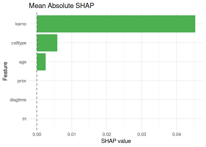
shap_meanabs <- compute_shap(
  model         = mod_cox,
  newdata       = veteran[100,],
  baseline_data = veteran,
  times         = 80,
  sample.size   = 50,
  aggregate     = TRUE,
  method        = "meanabs"
  )

shap_meanabs
#>           feature         phi
#> trt           trt 0.000000000
#> celltype celltype 0.005850095
#> karno       karno 0.045326970
#> diagtime diagtime 0.000000000
#> age           age 0.002540069
#> prior prior 0.000000000plot_shap(shap_meanabs)
survalis also provides PDP, ALE, surrogate explanations,
tree surrogates, permutation importance, interaction analysis, and
counterfactuals.
Partial dependence and ICE
pdp_age <- compute_pdp(
  model = mod_cox,
  data = veteran,
  feature = "age",
  times = c(100, 200, 300),
  method = "pdp+ice"
  )

plot_pdp(pdp_age, feature = "age", which = "per_time")
#> Warning: `aes_string()` was deprecated in ggplot2 3.0.0.
#> ℹ Please use tidy evaluation idioms with `aes()`.
#> ℹ See also `vignette("ggplot2-in-packages")` for more information.
#> ℹ The deprecated feature was likely used in the survalis package.
#>   Please report the issue to the authors.
#> This warning is displayed once per session.
#> Call `lifecycle::last_lifecycle_warnings()` to see where this warning was
#> generated.
#> Warning: Using `size` aesthetic for lines was deprecated in ggplot2 3.4.0.
#> ℹ Please use `linewidth` instead.
#> ℹ The deprecated feature was likely used in the survalis package.
#>   Please report the issue to the authors.
#> This warning is displayed once per session.
#> Call `lifecycle::last_lifecycle_warnings()` to see where this warning was
#> generated.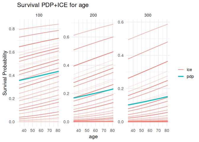
plot_pdp(pdp_age, feature = "age", which = "integrated", smooth = TRUE)
#> `geom_smooth()` using formula = 'y ~ x'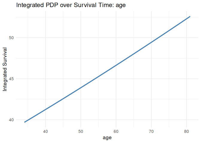
Accumulated local effects
ale_karno <- compute_ale(
  model = mod_cox,
  newdata = veteran,
  feature = "karno",
  times = c(100, 200, 300)
  )

plot_ale(ale_karno, feature = "karno", which = "per_time")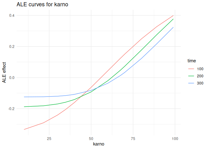
plot_ale(ale_karno, feature = "karno", which = "integrated", smooth = TRUE)
#> `geom_smooth()` using formula = 'y ~ x'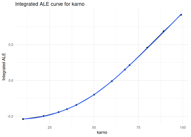
Local surrogate explanation
local_surrogate <- compute_surrogate(
  model = mod_cox,
  newdata = veteran[1, , drop = FALSE],
  baseline_data = veteran,
  times = c(100, 200, 300),
  target_time = 200,
  k = 5
  )

local_surrogate
#>    feature feature_value      effect target_time
#> 1    karno            60 0.491034890         200
#> 2 celltype      squamous 0.189632633         200
#> 3      age            69 0.120729843         200
#> 4 diagtime             7 0.001800378         200
#> 5    prior             0 0.000000000         200
plot_surrogate(local_surrogate, top_n = 10)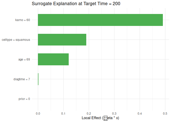
Tree surrogate
tree_surrogate <- compute_tree_surrogate(
  model = mod_cox,
  data = veteran,
  times = c(100, 200, 300)
  )

plot_tree_surrogate(tree_surrogate, type = "importance", top_n = 5)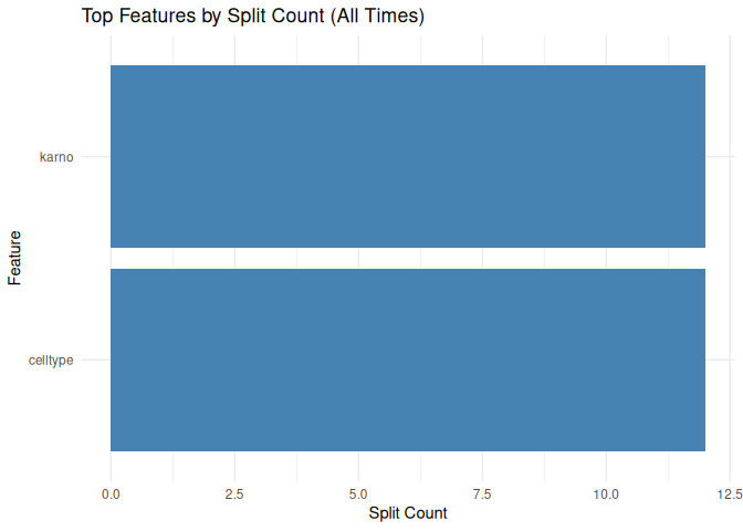
# plot_tree_surrogate(tree_surrogate, type = "tree")Permutation variable importance
varimp_res <- compute_varimp(
  model = mod_cox,
  times = c(100, 200, 300),
  metric = "ibs",
  n_repetitions = 5,
  seed = 123
  )

varimp_res
#> # A tibble: 6 × 5
#>   feature  importance importance_05 importance_95 scaled_importance
#>   <chr>         <dbl>         <dbl>         <dbl>             <dbl>
#> 1 karno       0.0624          0.192         0.223            100
#> 2 celltype    0.0446          0.185         0.201             71.5
#> 3 age        -0.00180         0.144         0.146              2.89
#> 4 trt         0               0.147         0.147              0
#> 5 diagtime    0               0.147         0.147              0
#> 6 prior       0               0.147         0.147              0
plot_varimp(varimp_res)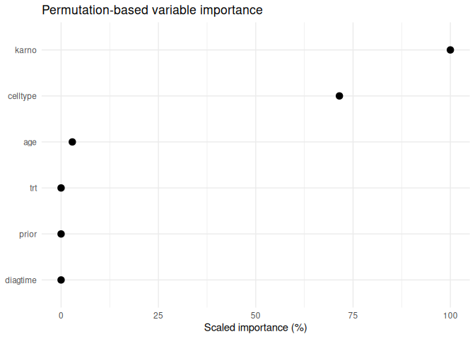
Feature interactions
interaction_1way <- compute_interactions(
  model = mod_cox,
  data = veteran,
  times = c(100, 200, 300),
  target_time = 200,
  type = "1way"
  )

interaction_heatmap <- compute_interactions(
  model = mod_cox,
  data = veteran,
  times = c(100, 200, 300),
  target_time = 200,
  type = "heatmap"
  )

interaction_time <- compute_interactions(
  model = mod_cox,
  data = veteran,
  times = c(100, 200, 300),
  type = "time"
  )

plot_interactions(interaction_1way, type = "1way")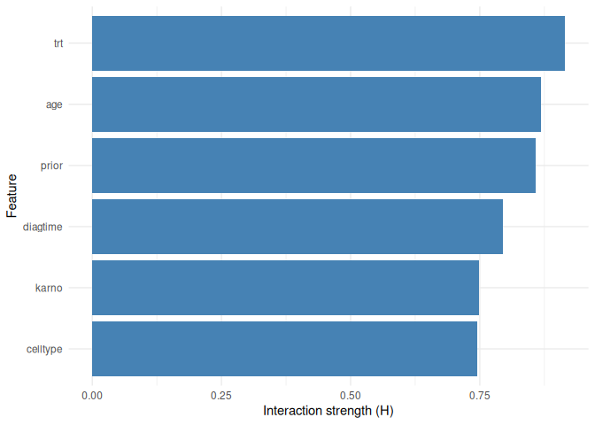
plot_interactions(interaction_heatmap, type = "heatmap")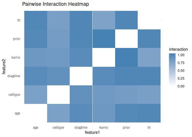
plot_interactions(interaction_time, type = "time")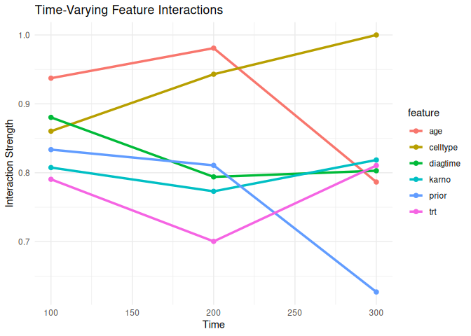
Counterfactual explanations
counterfactuals <- compute_counterfactual(
  model = mod_cox,
  newdata = veteran[1, , drop = FALSE],
  times = c(100, 200, 300),
  target_time = 200,
  features_to_change = c("age", "karno", "diagtime"),
  cost_penalty = 0.01
  )

counterfactuals
#>    feature original_value suggested_value survival_gain change_cost
#> 1    karno             60         81.0202        0.2347     21.0202
#> 2 diagtime              7          7.0808        0.0000      0.0808
#> 3      age             69         69.1313        0.0003      0.1313
#>   penalized_gain
#> 1         0.0245
#> 2        -0.0008
#> 3        -0.0010
5. Calibration
compute_calibration(
   model = mod_cox, data = veteran,
   time = "time", status = "status",
   eval_time = 80, n_bins = 10, n_boot = 30
   ) |> plot_calibration()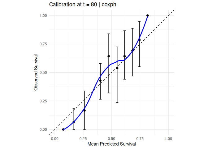
citation("survalis")These binaries (installable software) and packages are in development.
They may not be fully stable and should be used with caution. We make no claims about them.