The hardware and bandwidth for this mirror is donated by METANET, the Webhosting and Full Service-Cloud Provider.
If you wish to report a bug, or if you are interested in having us mirror your free-software or open-source project, please feel free to contact us at mirror[@]metanet.ch.
swjm implements stagewise (forward-stepwise) variable
selection for joint models of recurrent events and terminal events
(semi-competing risks). Two model frameworks are supported:
| Model | Type | alpha (first p) |
beta (second p) |
|---|---|---|---|
| JFM | Cox frailty | recurrence/readmission | terminal/death |
| JSCM | Scale-change (AFT) | recurrence/readmission | terminal/death |
Three penalty types are available: cooperative lasso
("coop"), lasso ("lasso"), and group lasso
("group"). The cooperative lasso encourages shared support
between the readmission and death coefficient vectors.
# From the package directory:
devtools::install("swjm")All functions expect a data frame with columns id,
t.start, t.stop, event (1 =
readmission, 0 = terminal/censoring row), status (1 =
death, 0 = alive/censored), and covariate columns
x1, ..., xp.
library(swjm)

# Joint Frailty Model — scenario 1
set.seed(42)
dat_jfm  <- generate_data(n = 200, p = 100, scenario = 1, model = "jfm")
Data_jfm <- dat_jfm$data

# JSCM — same scenario
set.seed(42)
dat_jscm  <- generate_data(n = 200, p = 100, scenario = 1, model = "jscm")
#> Call:
#> reReg::simGSC(n = n, summary = TRUE, para = para, xmat = X, censoring = C,
#>     frailty = gamma, tau = 60)
#>
#> Summary:
#> Sample size:                                    200
#> Number of recurrent event observed:             343
#> Average number of recurrent event per subject:  1.715
#> Proportion of subjects with a terminal event:   0.175
Data_jscm <- dat_jscm$data
JFM data: n = 200 subjects, 382 readmission events, 48 deaths
fit_jfm <- stagewise_fit(Data_jfm, model = "jfm", penalty = "coop")
fit_jfm
#> Stagewise path (jfm/coop)
#>
#>   Covariates (p):            100
#>   Iterations:                5000
#>   Lambda range:              [0.08902, 1.301]
#>   Active at final step:      44 readmission, 34 death
#>     Readmission (alpha): 1, 2, 3, 4, 5, 7, 9, 10, 12, 14, 15, 17, 23, 33, 35, 37, 38, 39, 41, 43, 47, 49, 52, 55, 57, 60, 62, 64, 66, 67, 69, 71, 73, 74, 77, 79, 80, 82, 92, 93, 95, 96, 97, 98
#>     Death (beta):        3, 4, 5, 7, 9, 10, 12, 14, 15, 17, 25, 37, 38, 39, 41, 43, 47, 49, 52, 57, 60, 62, 66, 67, 73, 74, 78, 80, 82, 84, 95, 96, 97, 98
The fit object now exposes alpha (readmission) and
beta (death) as separate p × (k+1)
matrices — one column per stagewise step — in addition to the combined
theta matrix (2p × (k+1)):
p <- 100
k_final <- ncol(fit_jfm$alpha)
a_final <- round(fit_jfm$alpha[, k_final], 4)Nonzero alpha entries at final step:
a_final[a_final != 0]
#>  [1]  1.0057 -0.9787  0.0183 -0.0577  0.0185  0.0151  0.9614 -0.8484  0.0124
#> [10]  0.0423 -0.0284  0.0199 -0.0020  0.0240 -0.0240  0.0064  0.0781 -0.0061
#> [19]  0.0125  0.0046 -0.0429  0.0396  0.0092  0.0680 -0.0550 -0.0500 -0.0007
#> [28]  0.0200  0.0742  0.0005 -0.0350  0.0370  0.0099 -0.0234  0.0450  0.0790
#> [37] -0.0072  0.0013 -0.0200  0.0150  0.0085  0.0027 -0.0618  0.0272
summary() shows a compact table of path-end coefficients
with variable type (shared, readmission-only, or death-only):
summary(fit_jfm)
#> Stagewise path (jfm/coop)
#>
#>   p = 100  |  5000 iterations  |  lambda: [0.08902, 1.301]
#>   Decreasing path: 784 steps
#>
#>   Path-end coefficients (nonzero variables):
#>
#>   Variable    alpha       beta        Type
#>   ----------  ----------  ----------  ----------------
#>   x9          +0.9614     +0.6629     shared (+)
#>   x4          -0.0577     -0.9979     shared (+)
#>   x10         -0.8484     -0.7274     shared (+)
#>   x2          -0.9787          —    readmission only
#>   x3          +0.0183     +0.8049     shared (+)
#>   x74         -0.0234     -0.3101     shared (+)
#>   x1          +1.0057          —    readmission only
#>   x67         +0.0005     +0.1393     shared (+)
#>   x57         -0.0550     +0.1330     shared (–)
#>   x38         +0.0781     +0.0857     shared (+)
#>   x97         -0.0618     -0.0583     shared (+)
#>   x66         +0.0742     +0.0415     shared (+)
#>   x41         +0.0125     +0.0937     shared (+)
#>   x55         +0.0680          —    readmission only
#>   x79         +0.0790          —    readmission only
#>   x60         -0.0500     +0.0070     shared (–)
#>   x49         +0.0396     +0.0305     shared (+)
#>   x98         +0.0272     +0.0792     shared (+)
#>   x15         -0.0284     -0.0639     shared (+)
#>   x7          +0.0151     +0.1160     shared (+)
#>   x82         +0.0013     +0.0750     shared (+)
#>   x5          +0.0185     +0.0527     shared (+)
#>   x39         -0.0061     -0.0657     shared (+)
#>   x14         +0.0423     +0.0076     shared (+)
#>   x47         -0.0429     -0.0135     shared (+)
#>   x71         +0.0370          —    readmission only
#>   x77         +0.0450          —    readmission only
#>   x69         -0.0350          —    readmission only
#>   x35         -0.0240          —    readmission only
#>   x33         +0.0240          —    readmission only
#>   x17         +0.0199     +0.0020     shared (+)
#>   x84              —    -0.0790     death only
#>   x37         +0.0064     +0.0394     shared (+)
#>   x78              —    +0.0710     death only
#>   x64         +0.0200          —    readmission only
#>   x92         -0.0200          —    readmission only
#>   x25              —    +0.0200     death only
#>   x80         -0.0072     -0.0165     shared (+)
#>   x93         +0.0150          —    readmission only
#>   x12         +0.0124     +0.0085     shared (+)
#>   x73         +0.0099     +0.0084     shared (+)
#>   x95         +0.0085     +0.0170     shared (+)
#>   x52         +0.0092     +0.0092     shared (+)
#>   x43         +0.0046     +0.0038     shared (+)
#>   x96         +0.0027     +0.0054     shared (+)
#>   x23         -0.0020          —    readmission only
#>   x62         -0.0007     -0.0007     shared (+)
#>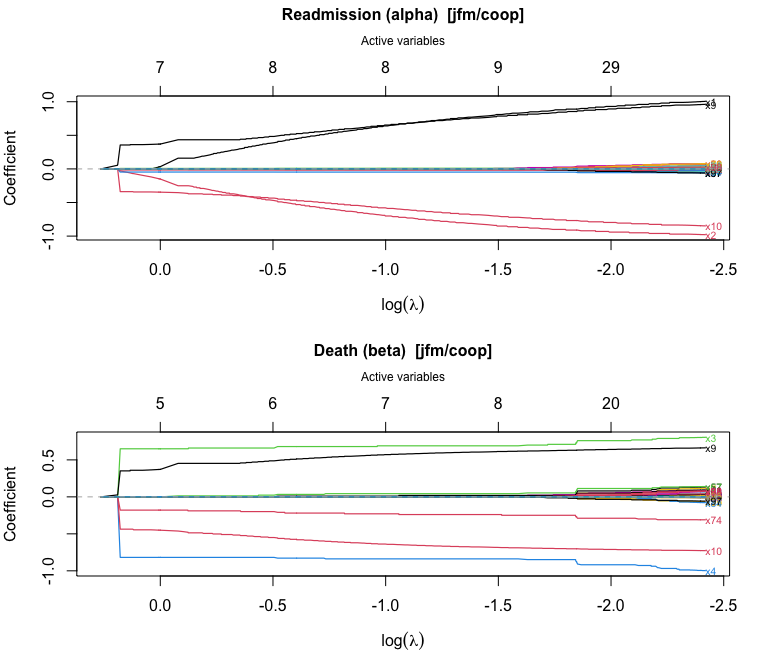
#> Inactive: x6, x8, x11, x13, x16, x18, x19, x20, x21, x22, x24, x26, x27, x28, x29, x30, x31, x32, x34, x36, x40, x42, x44, x45, x46, x48, x50, x51, x53, x54, x56, x58, x59, x61, x63, x65, x68, x70, x72, x75, x76, x81, x83, x85, x86, x87, x88, x89, x90, x91, x94, x99, x100plot() produces a glmnet-style coefficient trajectory
plot with the number of active variables on the top axis:
plot(fit_jfm)
cv_stagewise() evaluates a cross-fitted
estimating-equation score norm over a grid of lambda values.
lambda_path <- fit_jfm$lambda
dec_idx     <- swjm:::extract_decreasing_indices(lambda_path)
lambda_seq  <- lambda_path[dec_idx]

cv_jfm <- cv_stagewise(
  Data_jfm, model = "jfm", penalty = "coop",
  lambda_seq = lambda_seq, K = 3L
)
cv_jfm
#> Cross-validation (jfm/coop)
#>
#>   Covariates (p):              100
#>   Lambda grid size:            784
#>   Best position (combined):    438  (lambda = 0.9241)
#>   Selected variables:          8 readmission, 6 death
#>     Readmission (alpha): 1, 2, 3, 4, 9, 10, 67, 74
#>     Death (beta):        3, 4, 9, 10, 67, 74
The CV object stores alpha and beta at the
optimal lambda, plus n_active_alpha,
n_active_beta, and n_active variable-count
vectors across the full lambda grid.
plot(cv_jfm)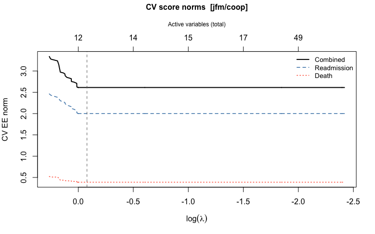
# summary() shows a formatted table of selected coefficients
summary(cv_jfm)
#> CV-selected model (jfm/coop)
#>
#>   p = 100  |  Lambda grid: 784 steps  |  CV optimal: step 438 (lambda = 0.9241)
#>
#>   Selected coefficients  (8 readmission, 6 death):
#>
#>   Variable    alpha       beta        Type
#>   ----------  ----------  ----------  ----------------
#>   x9          +0.4338     +0.4528     shared (+)
#>   x4          -0.0466     -0.8184     shared (+)
#>   x10         -0.3531     -0.4622     shared (+)
#>   x3          +0.0075     +0.6503     shared (+)
#>   x2          -0.2507          —    readmission only
#>   x74         -0.0162     -0.1793     shared (+)
#>   x1          +0.1597          —    readmission only
#>   x67         +0.0004     +0.0133     shared (+)
#>
#>   Inactive (92): x5, x6, x7, x8, x11, x12, x13, x14, x15, x16, x17, x18, x19, x20, x21, x22, x23, x24, x25, x26, x27, x28, x29, x30, x31, x32, x33, x34, x35, x36, x37, x38, x39, x40, x41, x42, x43, x44, x45, x46, x47, x48, x49, x50, x51, x52, x53, x54, x55, x56, x57, x58, x59, x60, x61, x62, x63, x64, x65, x66, x68, x69, x70, x71, x72, x73, x75, x76, x77, x78, x79, x80, x81, x82, x83, x84, x85, x86, x87, x88, x89, x90, x91, x92, x93, x94, x95, x96, x97, x98, x99, x100
Direct access to selected coefficients:
# coef() returns the combined numeric vector c(alpha, beta) for compatibility
theta_best <- coef(cv_jfm)baseline_hazard() evaluates the cumulative baseline
hazards at any desired time points (Breslow for JFM; Nelson-Aalen on the
accelerated scale for JSCM):
bh <- baseline_hazard(cv_jfm, times = c(0.5, 1.0, 2.0, 4.0, 6.0))
print(bh)
#>   time cumhaz_readmission cumhaz_death
#> 1  0.5          0.8302786   0.04821411
#> 2  1.0          1.3776457   0.06859515
#> 3  2.0          1.9078200   0.12461276
#> 4  4.0          3.1933429   0.28725353
#> 5 6.0 4.5481622 0.33588232predict() computes subject-specific readmission-free and
death-free survival curves, together with the per-predictor
contributions to each linear predictor:
# Three hypothetical new subjects (covariate vectors of length p = 100)
set.seed(7)
newz <- matrix(rnorm(300), nrow = 3, ncol = 100)
colnames(newz) <- paste0("x", 1:100)

pred <- predict(cv_jfm, newdata = newz)
pred
#> swjm predictions (jfm)
#>
#>   Subjects:                3
#>   Time points:             430
#>   Time range:              [0.0002844, 6.281]
#>
#>   Use plot() to visualize survival curves and predictor contributions.

# S_re: readmission-free survival — first 10 time points
round(pred$S_re[, 1:10], 3)
#>          t=0.0002844 t=0.0009392 t=0.001171 t=0.001381 t=0.001936 t=0.002432
#> Subject1       0.992       0.983      0.983      0.974      0.966      0.957
#> Subject2       0.994       0.987      0.987      0.980      0.973      0.967
#> Subject3       0.994       0.987      0.987      0.981      0.974      0.967
#>          t=0.004535 t=0.004809 t=0.006178 t=0.006205
#> Subject1      0.949      0.940      0.932      0.923
#> Subject2      0.960      0.953      0.947      0.940
#> Subject3      0.961      0.954      0.948      0.941

# Predictor contributions for subject 1 — show only nonzero entries
contrib1 <- round(pred$contrib_re[1, ], 3)
contrib1[contrib1 != 0]
#>     x1     x2     x3     x4     x9    x10    x74
#> 0.365 0.103 0.006 -0.102 0.552 -0.209 0.007plot() on a swjm_pred object draws four
panels: survival curves for both processes (all subjects in grey,
highlighted subject in color) plus bar charts of predictor contributions
for the selected subject.
plot(pred, which_subject = 1)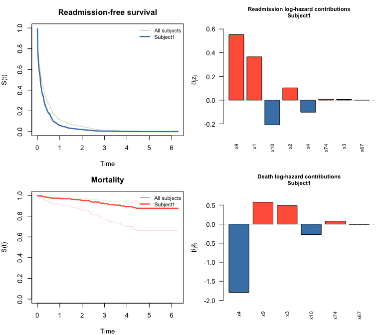
The same workflow applies to the JSCM. baseline_hazard()
and predict() now work for both models: for JSCM, survival
curves are estimated via a Nelson-Aalen baseline on the accelerated time
scale. In the AFT interpretation, \(e^{\hat\alpha^\top z_i}\) is the
time-acceleration factor for subject \(i\): greater than 1 means events happen
sooner, less than 1 means later.
fit_jscm <- stagewise_fit(Data_jscm, model = "jscm", penalty = "coop")

lambda_path_jscm <- fit_jscm$lambda
dec_idx_jscm     <- swjm:::extract_decreasing_indices(lambda_path_jscm)
lambda_seq_jscm  <- lambda_path_jscm[dec_idx_jscm]

cv_jscm <- cv_stagewise(
  Data_jscm, model = "jscm", penalty = "coop",
  lambda_seq = lambda_seq_jscm, K = 3L
)
summary(cv_jscm)
#> CV-selected model (jscm/coop)
#>
#>   p = 100  |  Lambda grid: 30 steps  |  CV optimal: step 3 (lambda = 0.6838)
#>
#>   Selected coefficients  (1 readmission, 1 death):
#>
#>   Variable    alpha       beta        Type
#>   ----------  ----------  ----------  ----------------
#>   x10         -0.0180     -0.0088     shared (+)
#>
#> Inactive (99): x1, x2, x3, x4, x5, x6, x7, x8, x9, x11, x12, x13, x14, x15, x16, x17, x18, x19, x20, x21, x22, x23, x24, x25, x26, x27, x28, x29, x30, x31, x32, x33, x34, x35, x36, x37, x38, x39, x40, x41, x42, x43, x44, x45, x46, x47, x48, x49, x50, x51, x52, x53, x54, x55, x56, x57, x58, x59, x60, x61, x62, x63, x64, x65, x66, x67, x68, x69, x70, x71, x72, x73, x74, x75, x76, x77, x78, x79, x80, x81, x82, x83, x84, x85, x86, x87, x88, x89, x90, x91, x92, x93, x94, x95, x96, x97, x98, x99, x100set.seed(7)
newz_jscm <- matrix(runif(600, -1, 1), nrow = 3, ncol = 100)
#> Warning in matrix(runif(600, -1, 1), nrow = 3, ncol = 100): data length differs
#> from size of matrix: [600 != 3 x 100]
pred_jscm <- predict(cv_jscm, newdata = newz_jscm)Recurrence time-acceleration factors:
round(pred_jscm$time_accel_re, 3)
#> Subject1 Subject2 Subject3
#>    1.000    0.983    1.005
plot() draws the same four-panel layout as for JFM:
survival curves for both processes plus bar charts of log
time-acceleration contributions.
plot(pred_jscm, which_subject = 1)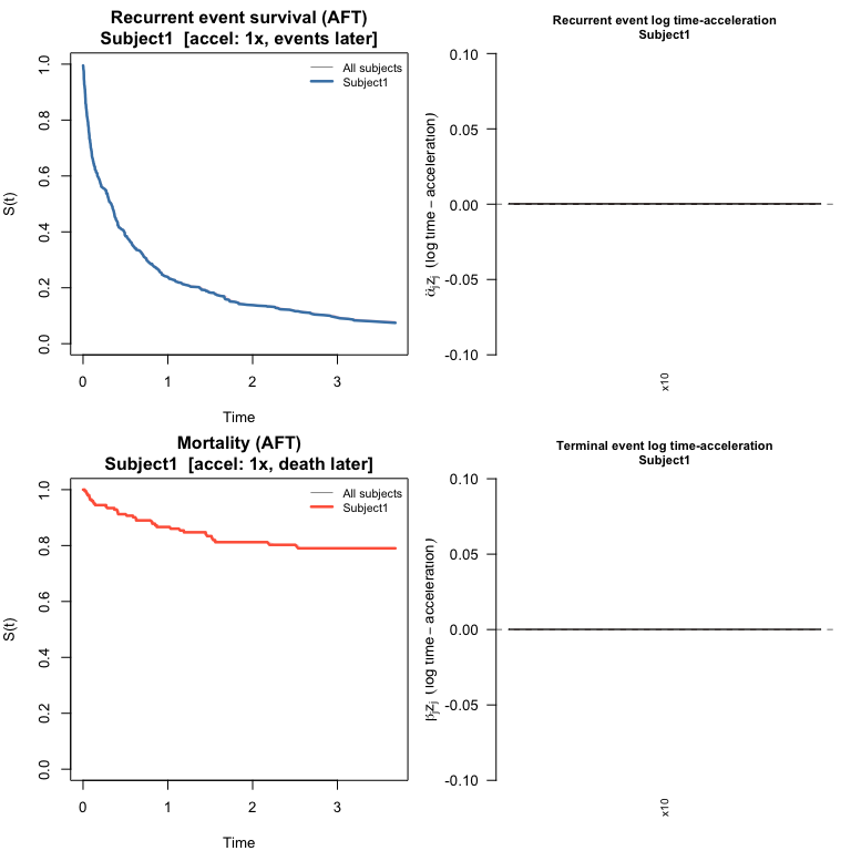
fit_lasso <- stagewise_fit(Data_jfm, model = "jfm", penalty = "lasso")
cv_lasso  <- cv_stagewise(Data_jfm, model = "jfm", penalty = "lasso", K = 3L)
summary(cv_lasso)

fit_group <- stagewise_fit(Data_jfm, model = "jfm", penalty = "group")
cv_group  <- cv_stagewise(Data_jfm, model = "jfm", penalty = "group", K = 3L)
summary(cv_group)Compare CV-optimal estimates to the true generating coefficients. Variables that are truly nonzero or were selected are shown; all others were correctly excluded.
p <- 100

# JFM: variables of interest (true signal or selected)
show_jfm <- sort(which(dat_jfm$alpha_true != 0 | cv_jfm$alpha != 0 |
                       dat_jfm$beta_true  != 0 | cv_jfm$beta  != 0))

coef_df <- data.frame(
  variable   = paste0("x", show_jfm),
  true_alpha = round(dat_jfm$alpha_true[show_jfm], 3),
  est_alpha  = round(cv_jfm$alpha[show_jfm],       3),
  true_beta  = round(dat_jfm$beta_true[show_jfm],  3),
  est_beta   = round(cv_jfm$beta[show_jfm],        3)
)
colnames(coef_df) <- c("variable", "alpha_true", "alpha_est", "beta_true", "beta_est")
print(coef_df, row.names = FALSE)
#>  variable alpha_true alpha_est beta_true beta_est
#>        x1        1.1     0.160       0.1    0.000
#>        x2       -1.1    -0.251      -0.1    0.000
#>        x3        0.1     0.007       1.1    0.650
#>        x4       -0.1    -0.047      -1.1   -0.818
#>        x9        1.0     0.434       1.0    0.453
#>       x10       -1.0    -0.353      -1.0   -0.462
#>       x67        0.0     0.000       0.0    0.013
#>       x74        0.0    -0.016       0.0   -0.179
JFM alpha: TP=6 FP=2 FN=0 | beta: TP=4 FP=2 FN=2
show_jscm <- sort(which(dat_jscm$alpha_true != 0 | cv_jscm$alpha != 0 |
                        dat_jscm$beta_true  != 0 | cv_jscm$beta  != 0))

coef_jscm <- data.frame(
  variable   = paste0("x", show_jscm),
  true_alpha = round(dat_jscm$alpha_true[show_jscm], 3),
  est_alpha  = round(cv_jscm$alpha[show_jscm],        3),
  true_beta  = round(dat_jscm$beta_true[show_jscm],  3),
  est_beta   = round(cv_jscm$beta[show_jscm],         3)
)
colnames(coef_jscm) <- c("variable", "alpha_true", "alpha_est", "beta_true", "beta_est")
print(coef_jscm, row.names = FALSE)
#>  variable alpha_true alpha_est beta_true beta_est
#>        x1        1.1     0.000       0.1    0.000
#>        x2       -1.1     0.000      -0.1    0.000
#>        x3        0.1     0.000       1.1    0.000
#>        x4       -0.1     0.000      -1.1    0.000
#>        x9        1.0     0.000       1.0    0.000
#>       x10       -1.0    -0.018      -1.0   -0.009
JSCM alpha: TP=1 FP=0 FN=5 | beta: TP=1 FP=0 FN=5
We use the timeROC package (Blanche et al., 2013) to
compute cause-specific time-varying AUC in the competing-risk framework.
Each subject contributes at most a first-readmission event (cause 1) and
a death event (cause 2). Each sub-model is assessed with its own linear
predictor: \(\hat\alpha^\top z_i\) for
readmission, \(\hat\beta^\top z_i\) for
death.
Note: AUC is evaluated on the training data for illustration. In practice use held-out or cross-validated predictions.
# Construct competing-risk dataset:
# Keep first readmission (event==1 & t.start==0) + death/censor (event==0).
# Status: 1 = first readmission, 2 = death, 0 = censored.
.cr_data <- function(Data) {
  d3 <- Data[Data$event == 0 | (Data$event == 1 & Data$t.start == 0), ]
  d3 <- d3[order(d3$id, d3$t.start, d3$t.stop), ]
  status <- ifelse(d3$event == 1 & d3$status == 0, 1L,
             ifelse(d3$event == 0 & d3$status == 0, 0L, 2L))
  list(data = d3, status = status)
}

cr_jfm  <- .cr_data(Data_jfm)
cr_jscm <- .cr_data(Data_jscm)

# Baseline covariates (one row per subject)
Z_jfm  <- as.matrix(Data_jfm[!duplicated(Data_jfm$id),   paste0("x", 1:p)])
Z_jscm <- as.matrix(Data_jscm[!duplicated(Data_jscm$id), paste0("x", 1:p)])

# Markers expanded to row level: alpha^T z for readmission, beta^T z for death
M_re_jfm  <- drop(Z_jfm  %*% cv_jfm$alpha)[cr_jfm$data$id]
M_de_jfm  <- drop(Z_jfm  %*% cv_jfm$beta)[cr_jfm$data$id]
M_re_jscm <- drop(Z_jscm %*% cv_jscm$alpha)[cr_jscm$data$id]
M_de_jscm <- drop(Z_jscm %*% cv_jscm$beta)[cr_jscm$data$id]
if (!requireNamespace("timeROC", quietly = TRUE))
install.packages("timeROC")
library(survival)
library(timeROC)
# Evaluation grid: 20 points spanning the 10th-85th percentile of event times
.tgrid <- function(t_vec, status, n = 20) {
t_ev <- t_vec[status > 0]
seq(quantile(t_ev, 0.10), quantile(t_ev, 0.85), length.out = n)
}
t_jfm <- .tgrid(cr_jfm$data$t.stop, cr_jfm$status)
t_jscm <- .tgrid(cr_jscm$data$t.stop, cr_jscm$status)
# Readmission AUC: alpha^T z marker, cause = 1
roc_re_jfm <- timeROC(T = cr_jfm$data$t.stop, delta = cr_jfm$status,
marker = M_re_jfm, cause = 1, weighting = "marginal",
times = t_jfm, ROC = FALSE, iid = FALSE)
roc_re_jscm <- timeROC(T = cr_jscm$data$t.stop, delta = cr_jscm$status,
marker = M_re_jscm, cause = 1, weighting = "marginal",
times = t_jscm, ROC = FALSE, iid = FALSE)
# Death AUC: beta^T z marker, cause = 2
roc_de_jfm <- timeROC(T = cr_jfm$data$t.stop, delta = cr_jfm$status,
marker = M_de_jfm, cause = 2, weighting = "marginal",
times = t_jfm, ROC = FALSE, iid = FALSE)
roc_de_jscm <- timeROC(T = cr_jscm$data$t.stop, delta = cr_jscm$status,
marker = M_de_jscm, cause = 2, weighting = "marginal",
times = t_jscm, ROC = FALSE, iid = FALSE).get_auc <- function(roc, cause) {
auc <- roc[[paste0("AUC_", cause)]]
if (is.null(auc)) auc <- roc$AUC
if (is.null(auc) || !is.numeric(auc)) return(rep(NA_real_, length(roc$times)))
if (length(auc) == length(roc$times) + 1) auc <- auc[-1]
as.numeric(auc)
}
old_par <- par(mfrow = c(1, 2), mar = c(4.5, 4, 3, 1))
plot(t_jfm, .get_auc(roc_re_jfm, 1), type = "l", lwd = 2, col = "steelblue",
xlab = "Time", ylab = "AUC(t)", main = "JFM", ylim = c(0.4, 1))
lines(t_jfm, .get_auc(roc_de_jfm, 2), lwd = 2, col = "tomato", lty = 2)
abline(h = 0.5, lty = 3, col = "grey60")
legend("bottomleft", c("Readmission", "Death"),
col = c("steelblue", "tomato"), lwd = 2, lty = c(1, 2),
bty = "n", cex = 0.85)
plot(t_jscm, .get_auc(roc_re_jscm, 1), type = "l", lwd = 2, col = "steelblue",
xlab = "Time", ylab = "AUC(t)", main = "JSCM", ylim = c(0.4, 1))
lines(t_jscm, .get_auc(roc_de_jscm, 2), lwd = 2, col = "tomato", lty = 2)
abline(h = 0.5, lty = 3, col = "grey60")
legend("bottomleft", c("Readmission", "Death"),
col = c("steelblue", "tomato"), lwd = 2, lty = c(1, 2),
bty = "n", cex = 0.85)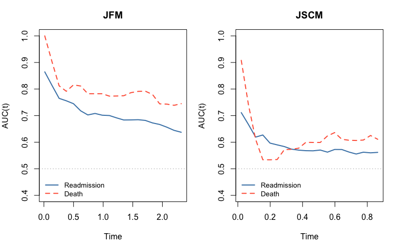
par(old_par)theta is always stored as
c(alpha, beta): theta[1:p] =
alpha (readmission), theta[(p+1):(2p)] =
beta (death). This holds for both the JFM and JSCM.stagewise_fit() also returns alpha and
beta as separate p × (k+1) matrices for
convenient access to the full regularization path.cv_stagewise() stores alpha and
beta at the CV-optimal lambda, plus variable-count vectors
n_active_alpha, n_active_beta,
n_active.cv$baseline and accessible via
baseline_hazard(cv, times). Works for both models: Breslow
estimator for JFM; Nelson-Aalen on the accelerated time scale for JSCM.
Used internally by predict().predict(cv, newdata) works for both models and returns a
swjm_pred object with S_re, S_de
(survival matrices), linear predictors lp_re,
lp_de, and predictor-contribution matrices
contrib_re, contrib_de (\(\hat\alpha_j z_{ij}\) and \(\hat\beta_j z_{ij}\)).
time_accel_re and
time_accel_de (\(e^{\hat\alpha^\top z_i}\), \(e^{\hat\beta^\top z_i}\)) — the
multiplicative factors by which each subject’s event times are scaled
relative to baseline. Contributions \(\hat\alpha_j z_{ij}\) are log
time-acceleration contributions: \(e^{\hat\alpha_j z_{ij}} > 1\) shortens
event times; \(< 1\) lengthens
them.(alpha_j, beta_j) with the L2 norm when signs agree,
and L1 when they disagree — encouraging variables that affect both
processes to enter together with the same sign.These binaries (installable software) and packages are in development.
They may not be fully stable and should be used with caution. We make no claims about them.