
The hardware and bandwidth for this mirror is donated by METANET, the Webhosting and Full Service-Cloud Provider.
If you wish to report a bug, or if you are interested in having us mirror your free-software or open-source project, please feel free to contact us at mirror[@]metanet.ch.
An R Package to generate data on tree architecture from terrestrial lidar scans
tReeTraits helps quantify tree architecture, especially
traits relevant to windfirmness (e.g., crown area, volume, stem taper,
branch size distribution), from individually segmented trees in
terrestrial lidar datasets.
It combines functionality from multiple tools including TreeQSM, PyTLidar, lidR, spanner, and follows methods described in Cannon et al. (in prep).
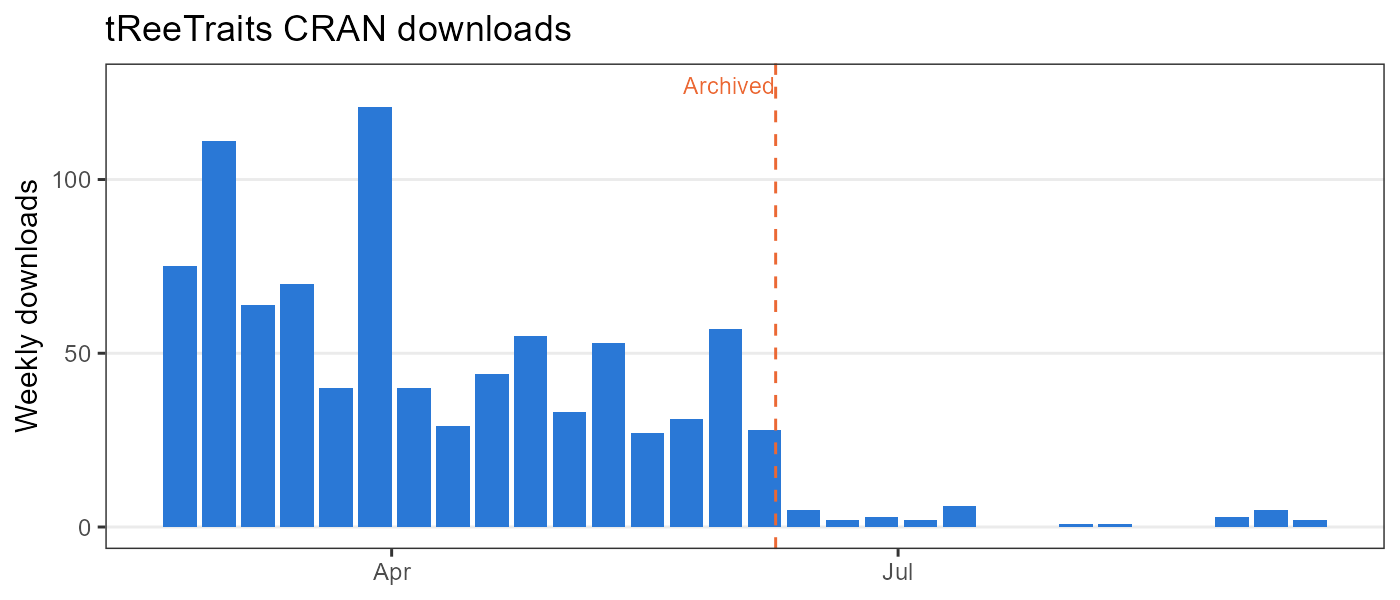
Weekly CRAN downloads (source: cranlogs; regenerate with
dev.R).
All dependencies (including lidR, spanner,
and CrownScorchTLS) are now available on CRAN:
```{r} install.packages(“tReeTraits”)
install.packages(“remotes”) devtools::install_github(“jbcannon/tReeTraits”)
## 🔧 Requirements (for QSM features)

### PyTLidar Setup (Run once per machine)

To use the TreeQSM functionality, you must have a conda environment named
`r-reticulate-pytlidar`, running **Python 3.11** with the **PyTLidar**
package and its dependencies installed.
This is handled automatically by the `setup_pytlidar()` function which must
be run once on each new machine.  Once installed the environment
is automatically detected when the package is loaded.

To enable TreeQSM functionality, run:

```{r}
setup_pytlidar()
This installs miniconda if needed, creates a dedicated Python environment, and installs PyTLidar and required dependencies.
The environment is automatically checked with each call to the
run_treeqsm function. If the environment is missing, you
will be prompted to run setup_pytlidar().
```{r}
library(tReeTraits) library(lidR)
las_filename = system.file(“extdata”, “tree_0744.laz”, package = “tReeTraits”) #las_filename = “C:/path/to/data/myfile.las” #or your own data las <- readLAS(las_filename)
las_clean <- clean_las(las, bole_height = 2)
plot_tree(las_clean)
<img src="man/figures/clean_las_ex.jpg" width="300"/>

Pine tree with vegetation around bole removed.

### Basic Trait Calcuation

```{r}
height <- get_height(las_clean)
width  <- get_width(las_clean)[1]
dbh    <- get_dbh(las_clean, select_n = 30)
cbh <- get_crown_base(las_clean, threshold = 0.25, sustain = 2)``{r} # first detect crown points withsegment_crown()`
las_crown <- segment_crown(las_clean, crown_base_height = cbh)
area_convex <- st_area(convex_hull_2D(las_crown)) area_voxel <- st_area(voxel_hull_2D(las_crown)) lacunarity <- get_lacunarity(las_crown) volume_alpha <- get_crown_volume_alpha(las_crown) volume_voxel <- get_crown_volume_voxel(las_crown)
<img src="man/figures/get_lacunarity.JPG" width="137"/>

Illustration of convex hull (dashed line) and voxel hull (green feature) from example tree. The proportion of whitespace within the convex hull represents lacunarity (\~20%)

### 🌲 Example: Running TreeQSM from tReeTraits to generate a Quantitative Structure Model (QSM)

This example shows how to generate a Quantitative Structure Model (QSM) from a single-tree point cloud using TreeQSM via `tReeTraits`.

#### Step 0. Ensure PyTLidar is available

```{r}
library(tReeTraits)

# Creates and manages an isolated Python environment if needed
setup_pytlidar()
# Note that you may need to Restart R to complete installation
# Only need to run once per machine{r} # Input file file <- system.file("extdata", "tree_0744.laz", package = "tReeTraits") tree_id <- tools::file_path_sans_ext(basename(file))
#### Step 2. Run TreeQSM
Multiple parameter combinations can be supplied. TreeQSM optimizes across them
{r} qsm_result <- run_treeqsm( file = file, intensity_threshold = 40000, resolution = 0.02, patch_diam1 = c(0.05, 0.1), patch_diam2min = c(0.04, 0.05), patch_diam2max = c(0.12, 0.14), verbose = TRUE )
```{r} # View the parameters of the best model params = qsm_result$qsm_pars print(params)
qsm = qsm_result$qsm plot_qsm2d(qsm, scale=40) #plot_qsm3d(qsm)
####  Step 4. Save results

```{r}
write_qsm(
  qsm_result,
  name = tree_id,
  output_dir = tempdir()
)
These functions analyze tree geometry and volume from Quantitative Structure Models (QSMs), enabling detailed trait extraction and modeling.
{r} qsm_file = system.file("extdata", "tree_0744_qsm.txt", package='tReeTraits') qsm = load_qsm(qsm_file)
Using the generated QSM, you can use the following functions for tree geometry traits
branch_volume_weighted_stats(qsm, breaks=NULL, FUN = mean)
Calculates volume-weighted branch diameter statistics using outputs from
branch_size_distribution().
get_primary_branches(qsm) Extracts primary branches
(branching order = 1 attached to trunk) from the QSM.
qsm_volume_distribution(qsm, terminus_diam_cm=4, segment_size=0.5)
Estimates tree volume and vertical distribution by separating trunk,
terminus (top trunk < terminus_diam_cm), and primary branches.
Returns diameters, heights, and volumes by section for further biomass
or mass-volume modeling.
fit_taper_Kozak(qsm, dbh, terminus_diam_cm=4, segment_size=0.25, plot=TRUE)
Fits Kozak’s taper equation to trunk segments, modeling diameter as a
function of relative height:
\[ d(h)/D = a_0 +a_1(h/H)+a_2(h/H)^2+a_3(h/H)^3 \]
Outputs model coefficients, R², RMSE, and an optional plot.
get_stem_sweep(qsm, terminus_diam_cm=4, plot=TRUE)
Computes tree sweep by measuring deviations of trunk points from a
straight idealized line between the top and bottom QSM trunk segments.
Returns sweep distances by height for quantifying stem curvature.
Optionally plots sweep vs. height.
get_stem_tilt(qsm, terminus_diam_cm=4) Calculates
overall stem tilt as the angle between the straight line connecting the
lowest and highest trunk points and the vertical axis. Outputs tilt
angle in degrees, quantifying tree lean.
This section provides functions to generate diagnostic plots that help visualize tree point clouds, QSMs, and related metrics to identify potential errors or assess data quality.
Creates a 3-panel plot showing two vertical profiles (X-Z and Y-Z) and an overhead (X-Y) view of the tree crown point cloud. Useful for spotting stray points or segmentation errors.
{r} plot_tree(las, res = 0.05, plot = TRUE)

Figure illustrating 3 views of tree_0129
Displays a simple base R plot of the QSM colored by branching order, optionally showing two rotated views.
{r} qsm_file = system.file("extdata", "tree_0744_qsm.txt", package='tReeTraits') qsm = load_qsm(qsm_file) plot_qsm2d(qsm) plot_qsm3d(qsm)

plot_qsm2d() and plot_qsm3d() output for
tree-0744
Visualizes basic tree measurements (height, crown base height, crown width, DBH) overlaid on a voxel-thinned point cloud.
{r} las_file = system.file("extdata", "tree_0744.laz", package="tReeTraits") las = lidR::readLAS(las_file) las = clean_las(las) basics_diagnostic_plot(las, height=24.1, cbh=13.9, crown_width=2.29, dbh=0.329, res = 0.1)

basics_diagnostic_plot() output for tree-0129
hull_diagnostic_plot(las, res = 0.1)taper_diagnostic_plot(qsm, dbh)branch_distribution_plot(qsm)full_diagnostic_plot(las, qsm, height, cbh, crown_width, dbh, res = 0.1)The treeTraits package is associated with Cannon et
al. (in press) XXXX. Please return at a later date for a full
citation.
These binaries (installable software) and packages are in development.
They may not be fully stable and should be used with caution. We make no claims about them.