The hardware and bandwidth for this mirror is donated by METANET, the Webhosting and Full Service-Cloud Provider.
If you wish to report a bug, or if you are interested in having us mirror your free-software or open-source project, please feel free to contact us at mirror[@]metanet.ch.

tauProcess

In clinical trials, nonproportional hazard (NPH) scenarios are commonly encountered. In such cases, the classical hazard ratio no longer serves as a meaningful treatment effect measure. Furthermore, the commonly-used logrank test may lose its power. To address these challenges, several treatment effect measures and testing procedures have been proposed, including weighted logrank, restricted mean survival time (RMST), and maxcombo tests. The proposed tau measures/processes are intuitive and clinically meaningful, in line with the requirements outlined in the addendum to ICH E9, which places emphasis on the interpretability of the estimand. For details, please refer to Tai, Wang and Wells (2023) https://doi.org/10.1002/pst.2324.

In immuno-oncology trials, it is often observed that Kaplan-Meier curves exhibit plateaus. This indicates the presence of a cure fraction or long-term survivors in the population. The mixture cure framework allows for separating the treatment effects on the cure fractions and the susceptible subgroups. Subsequently, this package also provides a function which can produce a tau process designed to measure the treatment effect over time for the susceptible subgroups. The cure rate for each group is estimated by the tail value of the Kaplan-Meier estimator.

Installation

You can install the development version of tauProcess from GitHub with:

# install.packages("devtools")
devtools::install_github("s07308/tauProcess")

Usage & Example

This is a basic example which shows you how to estimate the tau process and make the corresponding statistical inference:

library(tauProcess)
fit <- tau.fit(data = pbc)

You may use summary() to check the inference results at the largest time specified:

summary(fit)
#>  N0= 131  N1= 127  The truncation time is specified as 4523 
#> 
#> Random grouping design:
#>      tau   se(R)  z(R) Pr(>|z|) (R)
#>  -0.0503  0.0906 -0.55         0.58
#> 
#> Fixed grouping design:
#>      tau   se(F)  z(F) Pr(>|z|) (F)
#>  -0.0503  0.0906 -0.55         0.58
#> 
#>       tau lower .95(R) upper .95(R) lower .95(F) upper .95(F)
#>   -0.0503       -0.228        0.127       -0.228        0.127

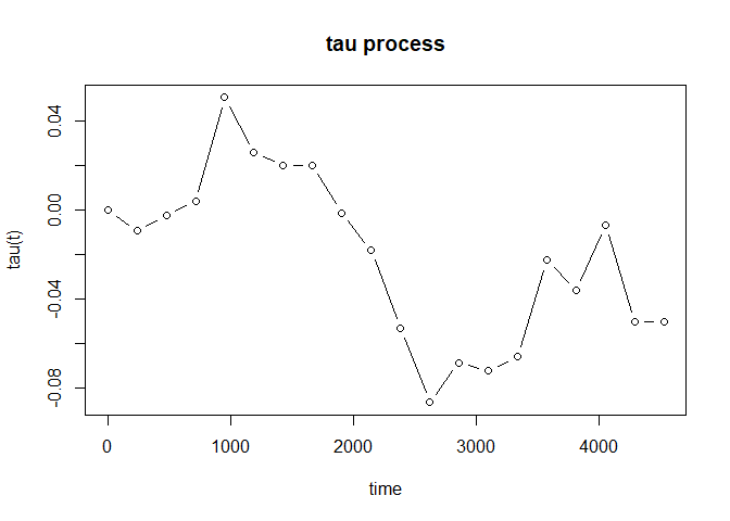
Furthermore, plot() will provide you the estimated tau process to investigate the evolution of treatment effect:

plot(fit, type = "b")

For the case with possibly existing cure fraction, we may estimate the tau process for the susceptible subgroups:

fit_cure <- tau_proc(pbc, cure = TRUE)

Bootstrap
The bootstrap method is recommended to make statistical inference about the tau process for susceptible subgroups. For given time point \(t\), we may make an inference on \(\tau_a(t)\). The p-value with respect to the null \(H_0: \tau_a(t) = 0\) may be calculated by the following steps:

# install.packages("boot")
library(boot)

boot_fun <- function(data, indices, t) {
  d <- data[indices, ]
  tau_fit <- tau_proc(d, t = t, cure = TRUE)
  
  tau_fit$vals_tau_proc
}

num_boot <- 5000
t <- 1000

boot_results <- boot(pbc, statistic = boot_fun, t = t, R = num_boot, strata = pbc$arm)
sd_est <- sd(boot_results$t)

pchisq((boot_results$t0 / sd_est) ^ 2, df = 1, lower.tail = FALSE)
#> [1] 0.2768823

If we let \(t = X_{(n_0)} \wedge X_{(n_1)}\), \(\hat{\tau}_a(t)\) can be treated as \(\hat{\tau}_a\) under sufficient follow-up. The p-value with respect to the null \(H_0: \tau_a = 0\) may be calculated by the following steps:

# install.packages("boot")
library(boot)

boot_fun <- function(data, indices) {
  d <- data[indices, ]
  tau_fit <- tau_proc(d, cure = TRUE)
  
  tail(tau_fit$vals_tau_proc, 1)
}

num_boot <- 5000

boot_results <- boot(pbc, statistic = boot_fun, R = num_boot, strata = pbc$arm)
sd_est <- sd(boot_results$t)

pchisq((boot_results$t0 / sd_est) ^ 2, df = 1, lower.tail = FALSE)
#> [1] 0.7988995

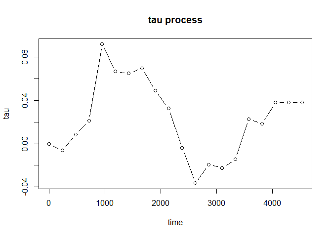
As the case with no cure fraction, we may plot the estimated tau process as well:

plot(fit_cure, type = "b")

These binaries (installable software) and packages are in development.
They may not be fully stable and should be used with caution. We make no claims about them.