The hardware and bandwidth for this mirror is donated by METANET, the Webhosting and Full Service-Cloud Provider.
If you wish to report a bug, or if you are interested in having us mirror your free-software or open-source project, please feel free to contact us at mirror[@]metanet.ch.

tidyfit is an R-package that facilitates
and automates linear and nonlinear regression and classification
modeling in a tidy environment. The package includes methods such as the
Lasso, PLS, time-varying parameter or Bayesian model averaging
regressions, and many more. The aim is threefold:
caret, the aim is not to cover a comprehensive set of
available packages, but rather a curated list of the most useful
ones.tidy data,
including verbs for regression and classification, automatic
consideration of grouped data, and tidy output formats
throughout.tidyfit builds on the tidymodels suite, but
emphasizes automated modeling with a focus on grouped data, model
comparisons, and high-volume analytics. The objective is to make model
fitting, cross validation and model output very simple and standardized
across all methods, with many necessary method-specific transformations
handled in the background.
tidyfit can be installed from CRAN or the development
version from GitHub
with:
# CRAN
install.packages("tidyfit")

# Dev version
# install.packages("devtools")
devtools::install_github("jpfitzinger/tidyfit")

library(tidyfit)tidyfit includes 3 deceptively simple functions:
regress()classify()m()All 3 of these functions return a tidyfit.models frame,
which is a data frame containing information about fitted regression and
classification models. regress and classify
perform regression and classification on tidy data. The functions ingest
a tibble, prepare input data for the models by splitting
groups, partitioning cross validation slices and handling any necessary
adjustments and transformations. The data is ultimately passed to the
model wrapper m() which fits the models.
To illustrate basic usage, suppose we would like to fit a financial factor regression for 10 industries with exponential weighting, comparing a WLS and a weighted LASSO regression:
progressr::handlers(global=TRUE)

tidyfit::Factor_Industry_Returns %>%
  group_by(Industry) %>%                       # Ensures that a model is fitted for each industry
  mutate(Weight = 0.96^seq(n(), 1)) %>%        # Exponential weights

  # 'regress' allows flexible standardized regression analysis in a single line of code
  regress(
    Return ~ .,                                # Uses normal formula syntax
    m("lasso"),                                # LASSO regression wrapper, 'lambda' grid set to default
    m("lm"),                                   # OLS wrapper (can add as many wrappers as necessary here)
    .cv = "initial_time_split",                # Cross-validation method for optimal 'lambda' in LASSO
    .mask = "Date",                            # 'Date' columns should be excluded
    .weights = "Weight"                        # Specifies the weights column
  ) -> models_df

# Get coefficients frame
coef(models_df)
The syntax is identical for classify.
m is a powerful wrapper for many different regression
and classification techniques that can be used with regress
and classify, or as a stand-alone function:
m(
  <method>,           # e.g. "lm" or "lasso"
  formula, data,      # not passed when used within regress or classify
  ...                 # Args passed to underlying method, e.g. to stats::lm for OLS regression
)
An important feature of m() is that all arguments can be
passed as vectors, allowing generalized hyperparameter tuning or
scenario analysis for any method:
m("lasso", lambda = seq(0, 1, by = 0.1))m("robust", method = c("M", "MM"))m("subset", method = c("forward", "backward"))m("glm", family = list(binomial(link="logit"), binomial(link="probit")))Arguments that are meant to be vectors (e.g. weights) are recognized by the function and not interpreted as grids.
tidyfittidyfit currently implements the following methods:
| Method | Name | Package | Regression | Classification |
|---|---|---|---|---|
| Linear (generalized) regression or classification | ||||
| OLS | lm |
stats
|
yes | no |
| GLS | glm |
stats
|
yes | yes |
| Robust regression (e.g. Huber loss) | robust |
MASS
|
yes | no |
| Quantile regression | quantile |
quantreg
|
yes | no |
| ANOVA | anova |
stats
|
yes | yes |
| Regression or classification with L1 and L2 penalties | ||||
| LASSO | lasso |
glmnet
|
yes | yes |
| Ridge | ridge |
glmnet
|
yes | yes |
| Group LASSO | group_lasso |
gglasso
|
yes | yes |
| Adaptive LASSO | adalasso |
glmnet
|
yes | yes |
| ElasticNet | enet |
glmnet
|
yes | yes |
| Machine Learning | ||||
| Gradient boosting regression | boost |
mboost
|
yes | yes |
| Support vector machine | svm |
e1071
|
yes | yes |
| Random forest | rf |
randomForest
|
yes | yes |
| Quantile random forest | quantile_rf |
quantregForest
|
yes | yes |
| Neural Network | nnet |
nnet
|
yes | no |
| Factor regressions | ||||
| Principal components regression | pcr |
pls
|
yes | no |
| Partial least squares | plsr |
pls
|
yes | no |
| Hierarchical feature regression | hfr |
hfr
|
yes | no |
| Subset selection | ||||
| Best subset selection | subset |
bestglm
|
yes | yes |
| Genetic Algorithm | genetic |
gaselect
|
yes | no |
| General-to-specific | gets |
gets
|
yes | no |
| Bayesian regression | ||||
| Bayesian regression | bayes |
arm
|
yes | yes |
| Bayesian Ridge | bridge |
monomvn
|
yes | no |
| Bayesian Lasso | blasso |
monomvn
|
yes | no |
| Bayesian model averaging | bma |
BMS
|
yes | no |
| Bayesian Spike and Slab | spikeslab |
BoomSpikeSlab
|
yes | yes |
| Bayesian time-varying parameters regression | tvp |
shrinkTVP
|
yes | no |
| Mixed-effects modeling | ||||
| Generalized mixed-effects regression | glmm |
lme4
|
yes | yes |
| Specialized time series methods | ||||
| Markov-switching regression | mslm |
MSwM
|
yes | no |
| Feature selection | ||||
| Pearson correlation | cor |
stats
|
no | no |
| Chi-squared test | chisq |
stats
|
yes | yes |
| Minimum redundancy, maximum relevance | mrmr |
mRMRe
|
yes | yes |
| ReliefF | relief |
CORElearn
|
yes | yes |
See ?m for additional information.
It is important to note that the above list is not complete, since
some of the methods encompass multiple algorithms. For instance,
“subset” can be used to perform forward, backward or exhaustive search
selection using leaps. Similarly, “lasso” includes certain
grouped LASSO implementations that can be fitted with
glmnet.
In this section, a minimal workflow is used to demonstrate how the package works. For more detailed guides of specialized topics, or simply for further reading, follow these links:
tidyfit includes a data set of financial Fama-French
factor returns freely available here.
The data set includes monthly industry returns for 10 industries, as
well as monthly factor returns for 5 factors:
data <- tidyfit::Factor_Industry_Returns

# Calculate excess return
data <- data %>%
  mutate(Return = Return - RF) %>%
  select(-RF)

data
#> # A tibble: 7,080 × 8
#>      Date Industry Return `Mkt-RF`   SMB   HML   RMW   CMA
#>     <dbl> <chr>     <dbl>    <dbl> <dbl> <dbl> <dbl> <dbl>
#>  1 196307 NoDur     -0.76    -0.39 -0.44 -0.89  0.68 -1.23
#>  2 196308 NoDur      4.64     5.07 -0.75  1.68  0.36 -0.34
#>  3 196309 NoDur     -1.96    -1.57 -0.55  0.08 -0.71  0.29
#>  4 196310 NoDur      2.36     2.53 -1.37 -0.14  2.8  -2.02
#>  5 196311 NoDur     -1.4     -0.85 -0.89  1.81 -0.51  2.31
#>  6 196312 NoDur      2.52     1.83 -2.07 -0.08  0.03 -0.04
#>  7 196401 NoDur      0.49     2.24  0.11  1.47  0.17  1.51
#>  8 196402 NoDur      1.61     1.54  0.3   2.74 -0.05  0.9
#>  9 196403 NoDur      2.77     1.41  1.36  3.36 -2.21  3.19
#> 10 196404 NoDur     -0.77     0.1  -1.59 -0.58 -1.27 -1.04
#> # ℹ 7,070 more rows
We will only use a subset of the data to keep things simple:
df_train <- data %>%
  filter(Date > 201800 & Date < 202000)
df_test <- data %>%
  filter(Date >= 202000)
Before beginning with the estimation, we can activate the progress
bar visualization. This allows us to gauge estimation progress along the
way. tidyfit uses the progressr-package
internally to generate a progress bar — run
progressr::handlers(global=TRUE) to activate progress bars
in your environment.
For purposes of this demonstration, the objective will be to fit an
ElasticNet regression for each industry group, and compare results to a
robust least squares regression. This can be done with
regress after grouping the data. For grouped data, the
functions regress and classify estimate models
for each group independently:
model_frame <- df_train %>%
  group_by(Industry) %>%
  regress(Return ~ .,
          m("enet"),
          m("robust", method = "MM", psi = MASS::psi.huber),
          .cv = "initial_time_split", .mask = "Date")
Note that the penalty and mixing parameters are chosen automatically
using a time series train/test split
(rsample::initial_time_split), with a hyperparameter grid
set by the package dials. See ?regress for
additional CV methods. A custom grid can easily be passed using
lambda = c(...) and/or alpha = c(...) in the
m("enet") wrapper.
The resulting tidyfit.models frame consists of 3
components:
Industry column, the model name, and grid ID (the ID for
the model settings used).estimator_fct, size (MB) and
model_object columns. These columns contain information on
the model itself. The model_object is the fitted
tidyFit model (an R6 class that contains the
model object as well as any additional information needed to perform
predictions or access coefficients)settings, as well as (if applicable)
messages and warnings.subset_mod_frame <- model_frame %>%
filter(Industry %in% unique(Industry)[1:2])
subset_mod_frame
#> # A tibble: 4 × 8
#> Industry model estimator_fct `size (MB)` grid_id model_object settings
#> <chr> <chr> <chr> <dbl> <chr> <list> <list>
#> 1 Enrgy enet glmnet::glmnet 1.21 #001|100 <tidyFit> <tibble>
#> 2 Shops enet glmnet::glmnet 1.21 #001|049 <tidyFit> <tibble>
#> 3 Enrgy robust MASS::rlm 0.0638 #0010000 <tidyFit> <tibble>
#> 4 Shops robust MASS::rlm 0.0638 #0010000 <tidyFit> <tibble>
#> # ℹ 1 more variable: warnings <chr>Let’s unnest the settings columns:
subset_mod_frame %>%
  tidyr::unnest(settings, keep_empty = TRUE)
#> # A tibble: 4 × 13
#>   Industry model  estimator_fct  `size (MB)` grid_id  model_object alpha weights
#>   <chr>    <chr>  <chr>                <dbl> <chr>    <list>       <dbl> <list>
#> 1 Enrgy    enet   glmnet::glmnet      1.21   #001|100 <tidyFit>        0 <NULL>
#> 2 Shops    enet   glmnet::glmnet      1.21   #001|049 <tidyFit>        0 <NULL>
#> 3 Enrgy    robust MASS::rlm           0.0638 #0010000 <tidyFit>       NA <NULL>
#> 4 Shops    robust MASS::rlm           0.0638 #0010000 <tidyFit>       NA <NULL>
#> # ℹ 5 more variables: family <chr>, lambda <dbl>, method <chr>, psi <list>,
#> #   warnings <chr>
The tidyfit.models frame can be used to access
additional information. Specifically, we can do 4 things:
The fitted tidyFit models are stored as an
R6 class in the model_object column and can be
addressed directly with generics such as coef or
summary. The underlying object (e.g. an lm
class fitted model) is given in ...$object (see here
for another example):
subset_mod_frame %>%
  mutate(fitted_model = map(model_object, ~.$object))
#> # A tibble: 4 × 9
#>   Industry model  estimator_fct  `size (MB)` grid_id  model_object settings
#>   <chr>    <chr>  <chr>                <dbl> <chr>    <list>       <list>
#> 1 Enrgy    enet   glmnet::glmnet      1.21   #001|100 <tidyFit>    <tibble>
#> 2 Shops    enet   glmnet::glmnet      1.21   #001|049 <tidyFit>    <tibble>
#> 3 Enrgy    robust MASS::rlm           0.0638 #0010000 <tidyFit>    <tibble>
#> 4 Shops    robust MASS::rlm           0.0638 #0010000 <tidyFit>    <tibble>
#> # ℹ 2 more variables: warnings <chr>, fitted_model <list>
To predict, we need data with the same columns as
the input data and simply use the generic predict function.
Groups are respected and if the response variable is in the data, it is
included as a truth column in the resulting object:
predict(subset_mod_frame, data)
#> # A tibble: 2,832 × 4
#> # Groups:   Industry, model [4]
#>    Industry model prediction truth
#>    <chr>    <chr>      <dbl> <dbl>
#>  1 Enrgy    enet      -3.77   2.02
#>  2 Enrgy    enet       3.90   3.69
#>  3 Enrgy    enet      -2.40  -3.91
#>  4 Enrgy    enet      -3.30  -0.61
#>  5 Enrgy    enet       0.762 -1.43
#>  6 Enrgy    enet      -0.293  4.36
#>  7 Enrgy    enet       3.68   4.54
#>  8 Enrgy    enet       2.31   0.8
#>  9 Enrgy    enet       7.26   1.09
#> 10 Enrgy    enet      -2.53   3.74
#> # ℹ 2,822 more rows
Finally, we can obtain a tidy frame of the
coefficients using the generic coef function:
estimates <- coef(subset_mod_frame)
estimates
#> # A tibble: 24 × 5
#> # Groups:   Industry, model [4]
#>    Industry model term        estimate model_info
#>    <chr>    <chr> <chr>          <dbl> <list>
#>  1 Enrgy    enet  (Intercept) -0.955   <tibble [1 × 4]>
#>  2 Enrgy    enet  Mkt-RF       1.20    <tibble [1 × 4]>
#>  3 Enrgy    enet  SMB          0.703   <tibble [1 × 4]>
#>  4 Enrgy    enet  HML         -0.00208 <tibble [1 × 4]>
#>  5 Enrgy    enet  RMW         -0.622   <tibble [1 × 4]>
#>  6 Enrgy    enet  CMA          1.32    <tibble [1 × 4]>
#>  7 Shops    enet  (Intercept)  1.03    <tibble [1 × 4]>
#>  8 Shops    enet  Mkt-RF       0.0849  <tibble [1 × 4]>
#>  9 Shops    enet  SMB          0.0353  <tibble [1 × 4]>
#> 10 Shops    enet  HML         -0.0149  <tibble [1 × 4]>
#> # ℹ 14 more rows
The estimates contain additional method-specific information that is
nested in model_info. This can include standard errors,
t-values and similar information:
tidyr::unnest(estimates, model_info)
#> # A tibble: 24 × 8
#> # Groups:   Industry, model [4]
#>    Industry model term        estimate lambda dev.ratio std.error statistic
#>    <chr>    <chr> <chr>          <dbl>  <dbl>     <dbl>     <dbl>     <dbl>
#>  1 Enrgy    enet  (Intercept) -0.955    0.536     0.812        NA        NA
#>  2 Enrgy    enet  Mkt-RF       1.20     0.536     0.812        NA        NA
#>  3 Enrgy    enet  SMB          0.703    0.536     0.812        NA        NA
#>  4 Enrgy    enet  HML         -0.00208  0.536     0.812        NA        NA
#>  5 Enrgy    enet  RMW         -0.622    0.536     0.812        NA        NA
#>  6 Enrgy    enet  CMA          1.32     0.536     0.812        NA        NA
#>  7 Shops    enet  (Intercept)  1.03    50.1       0.173        NA        NA
#>  8 Shops    enet  Mkt-RF       0.0849  50.1       0.173        NA        NA
#>  9 Shops    enet  SMB          0.0353  50.1       0.173        NA        NA
#> 10 Shops    enet  HML         -0.0149  50.1       0.173        NA        NA
#> # ℹ 14 more rows
Additional generics such as fitted or resid
can be used to obtain more information on the models.
Suppose we would like to evaluate the relative performance of the two
methods. This becomes exceedingly simple using the
yardstick package:
model_frame %>%
  # Generate predictions
  predict(df_test) %>%
  # Calculate RMSE
  yardstick::rmse(truth, prediction) %>%
  # Plot
  ggplot(aes(Industry, .estimate)) +
  geom_col(aes(fill = model), position = position_dodge())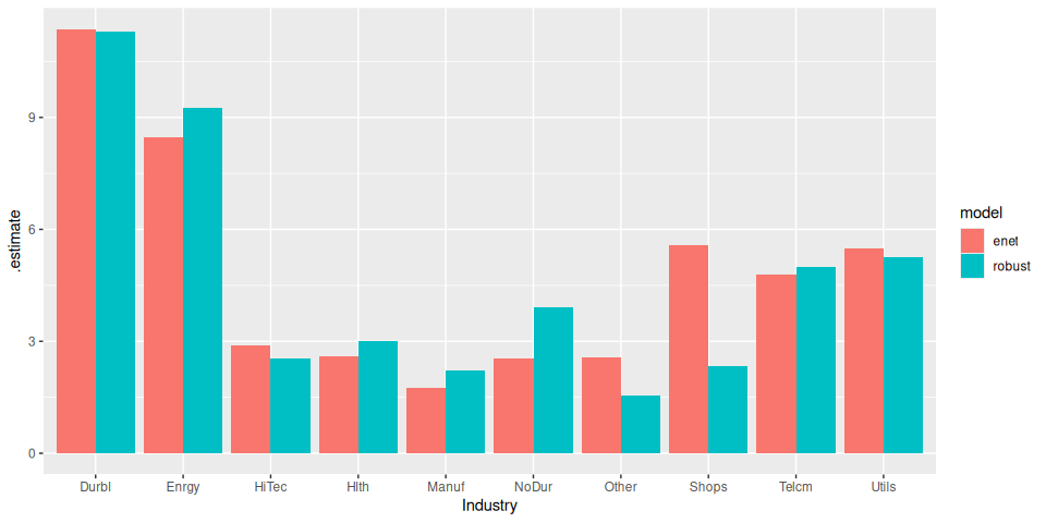
The ElasticNet performs a little better (unsurprising really, given the small data set).
A more detailed regression analysis of Boston house price data using a panel of regularized regression estimators can be found here.
These binaries (installable software) and packages are in development.
They may not be fully stable and should be used with caution. We make no claims about them.