The hardware and bandwidth for this mirror is donated by METANET, the Webhosting and Full Service-Cloud Provider.
If you wish to report a bug, or if you are interested in having us mirror your free-software or open-source project, please feel free to contact us at mirror[@]metanet.ch.
visOmopResults offers a set of functions tailored to
format objects of class <summarised_result>
(as
defined in omopgenerics
package).
It provides functionality to: transform data, create table visualizations, and generate plot visualizations. These visualizations are highly versatile for reporting results through Shiny apps, RMarkdown, Quarto, and more, supporting various output formats such as HTML, PNG, Word, and PDF.
You can install the latest version of visOmopResults from CRAN:
install.packages("visOmopResults")
Or you can install the development version from GitHub with:
# install.packages("pak")
::pkg_install("darwin-eu/visOmopResults") pak
The <summarised_result>
is a standardised output
format utilized across various packages, including:
Although this standard output format is essential, it can sometimes be challenging to manage. The visOmopResults package aims to simplify this process. To demonstrate the package’s functionality, let’s start by using some mock result:
library(visOmopResults)
<- mockSummarisedResult() result
<summarised_result>
objectA tidy version of the summarised can be obtained with the tidy function:
tidy(result)
#> # A tibble: 72 × 13
#> cdm_name cohort_name age_group sex variable_name variable_level count
#> <chr> <chr> <chr> <chr> <chr> <chr> <int>
#> 1 mock cohort1 overall overall number subjects <NA> 8073003
#> 2 mock cohort1 <40 Male number subjects <NA> 8850788
#> 3 mock cohort1 >=40 Male number subjects <NA> 3811096
#> 4 mock cohort1 <40 Female number subjects <NA> 7230087
#> 5 mock cohort1 >=40 Female number subjects <NA> 6508723
#> 6 mock cohort1 overall Male number subjects <NA> 7643684
#> 7 mock cohort1 overall Female number subjects <NA> 4209114
#> 8 mock cohort1 <40 overall number subjects <NA> 5850048
#> 9 mock cohort1 >=40 overall number subjects <NA> 8239237
#> 10 mock cohort2 overall overall number subjects <NA> 7597918
#> # ℹ 62 more rows
#> # ℹ 6 more variables: mean <dbl>, sd <dbl>, percentage <dbl>,
#> # result_type <chr>, package_name <chr>, package_version <chr>
This tidy format is no longer standardized but offers easier
manipulation. While tidy()
provides a straightforward
transformation, the more customizable sibling function
tidySummarisedResult()
allows you to specify exactly how
you’d like to tidy your <summarised_result>
object:
|>
result tidySummarisedResult(
splitStrata = FALSE,
settingsColumns = "package_name",
pivotEstimatesBy = NULL
)#> # A tibble: 126 × 11
#> result_id cdm_name cohort_name strata_name strata_level variable_name
#> <int> <chr> <chr> <chr> <chr> <chr>
#> 1 1 mock cohort1 overall overall number subje…
#> 2 1 mock cohort1 age_group &&& sex <40 &&& Male number subje…
#> 3 1 mock cohort1 age_group &&& sex >=40 &&& Male number subje…
#> 4 1 mock cohort1 age_group &&& sex <40 &&& Female number subje…
#> 5 1 mock cohort1 age_group &&& sex >=40 &&& Fema… number subje…
#> 6 1 mock cohort1 sex Male number subje…
#> 7 1 mock cohort1 sex Female number subje…
#> 8 1 mock cohort1 age_group <40 number subje…
#> 9 1 mock cohort1 age_group >=40 number subje…
#> 10 1 mock cohort2 overall overall number subje…
#> # ℹ 116 more rows
#> # ℹ 5 more variables: variable_level <chr>, estimate_name <chr>,
#> # estimate_type <chr>, estimate_value <chr>, package_name <chr>
<summarised_result>
objectA <summarised_result>
object is essentially a
<data.frame>
, so it can be filtered easily using
dplyr::filter()
. However, filtering variables within
name-level structures or those present in the settings can be
challenging. The following functions simplify this process:
filterSettings()
filterGroup()
filterStrata()
filterAdditional()
Here are some examples on how to use them:
|>
result filterSettings(package_name == "visOmopResults")
#> # A tibble: 126 × 13
#> result_id cdm_name group_name group_level strata_name strata_level
#> <int> <chr> <chr> <chr> <chr> <chr>
#> 1 1 mock cohort_name cohort1 overall overall
#> 2 1 mock cohort_name cohort1 age_group &&& sex <40 &&& Male
#> 3 1 mock cohort_name cohort1 age_group &&& sex >=40 &&& Male
#> 4 1 mock cohort_name cohort1 age_group &&& sex <40 &&& Female
#> 5 1 mock cohort_name cohort1 age_group &&& sex >=40 &&& Female
#> 6 1 mock cohort_name cohort1 sex Male
#> 7 1 mock cohort_name cohort1 sex Female
#> 8 1 mock cohort_name cohort1 age_group <40
#> 9 1 mock cohort_name cohort1 age_group >=40
#> 10 1 mock cohort_name cohort2 overall overall
#> # ℹ 116 more rows
#> # ℹ 7 more variables: variable_name <chr>, variable_level <chr>,
#> # estimate_name <chr>, estimate_type <chr>, estimate_value <chr>,
#> # additional_name <chr>, additional_level <chr>
|>
result filterSettings(package_name == "other")
#> # A tibble: 0 × 13
#> # ℹ 13 variables: result_id <int>, cdm_name <chr>, group_name <chr>,
#> # group_level <chr>, strata_name <chr>, strata_level <chr>,
#> # variable_name <chr>, variable_level <chr>, estimate_name <chr>,
#> # estimate_type <chr>, estimate_value <chr>, additional_name <chr>,
#> # additional_level <chr>
|>
result filterStrata(sex == "Female")
#> # A tibble: 42 × 13
#> result_id cdm_name group_name group_level strata_name strata_level
#> <int> <chr> <chr> <chr> <chr> <chr>
#> 1 1 mock cohort_name cohort1 age_group &&& sex <40 &&& Female
#> 2 1 mock cohort_name cohort1 age_group &&& sex >=40 &&& Female
#> 3 1 mock cohort_name cohort1 sex Female
#> 4 1 mock cohort_name cohort2 age_group &&& sex <40 &&& Female
#> 5 1 mock cohort_name cohort2 age_group &&& sex >=40 &&& Female
#> 6 1 mock cohort_name cohort2 sex Female
#> 7 1 mock cohort_name cohort1 age_group &&& sex <40 &&& Female
#> 8 1 mock cohort_name cohort1 age_group &&& sex >=40 &&& Female
#> 9 1 mock cohort_name cohort1 sex Female
#> 10 1 mock cohort_name cohort2 age_group &&& sex <40 &&& Female
#> # ℹ 32 more rows
#> # ℹ 7 more variables: variable_name <chr>, variable_level <chr>,
#> # estimate_name <chr>, estimate_type <chr>, estimate_value <chr>,
#> # additional_name <chr>, additional_level <chr>
Currently all table functionalities are built around 3 packages: tibble, gt, and flextable.
There are two main functions:
visOmopTable()
: Creates a well-formatted table
specifically from a <summarised_result>
object.visTable()
: Creates a nicely formatted table from any
<data.frame>
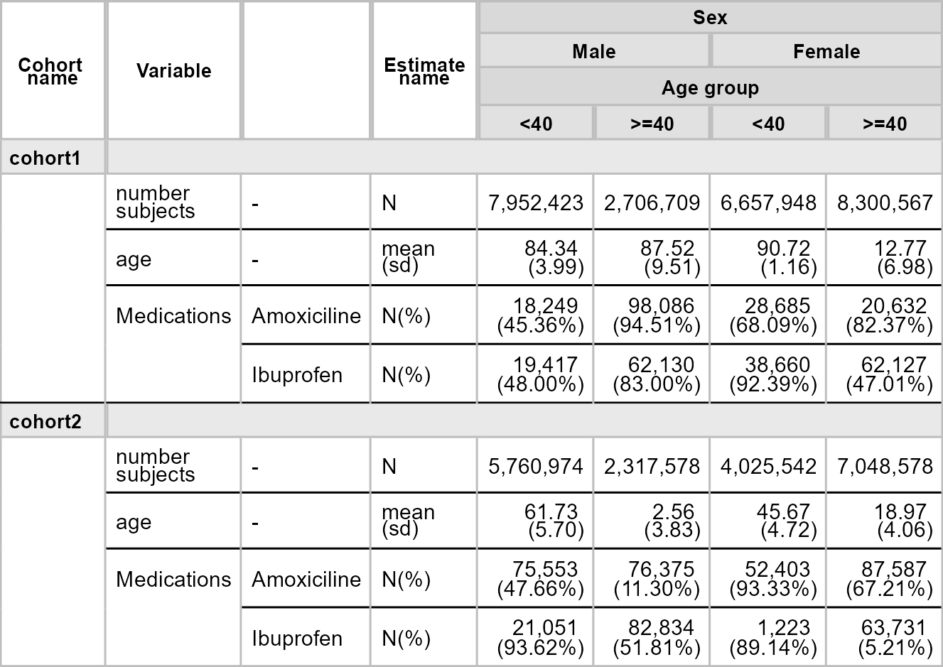
object.Let’s see a simple example:
|>
result visOmopTable(
type = "flextable", # to change to gt when issue 223 is fixed
estimateName = c(
"N(%)" = "<count> (<percentage>%)",
"N" = "<count>",
"mean (sd)" = "<mean> (<sd>)"),
header = c("sex"),
settingsColumns = NULL,
groupColumn = c("cohort_name", "age_group"),
rename = c("Variable" = "variable_name", " " = "variable_level"),
hide = "cdm_name"
)
Currently all plot functionalities are built around ggplot2. The
output of these plot functions is a <ggplot2>
object
that can be further customised.
There are three plotting functions:
plotScatter()
to create a scatter plot.plotBar()
to create a bar plot.plotBox()
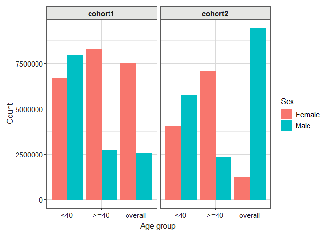
to create a box plot.Let’s see how we can create a simple boxplot for age using this tool:
library(dplyr)
|>
result filter(variable_name == "number subjects") |>
filterStrata(sex != "overall") |>
barPlot(x = "age_group",
y = "count",
facet = "cohort_name",
colour = "sex")
These binaries (installable software) and packages are in development.
They may not be fully stable and should be used with caution. We make no claims about them.