The hardware and bandwidth for this mirror is donated by METANET, the Webhosting and Full Service-Cloud Provider.
If you wish to report a bug, or if you are interested in having us mirror your free-software or open-source project, please feel free to contact us at mirror[@]metanet.ch.

windfarmGA

A genetic algorithm to optimize the layout of wind farms.

Version 5.0.0 uses a combinatorial genome (n unique grid-cell IDs), adaptive operator rates, and a memetic neighbourhood search on elites. The design, the north-wind gold layout, and the sensitivity results are documented in inst/reports/memetic-layout-ga.md.

Installation

The latest version can be installed from GitHub with:

devtools::install_github("YsoSirius/windfarmGA")
install.packages("windfarmGA")

Description

The genetic algorithm is designed to optimize wind farms of any shape. It requires a predefined number of turbines, a uniform rotor radius and an average wind speed per wind direction. It can include a terrain effect model, which requires an elevation raster and a surface roughness raster. The elevation data is used to find mountains and valleys and to adjust the wind speeds accordingly by ‘wind multipliers’ and to determine the air densities at rotor heights. The surface roughness raster with an additional elevation roughness value is used to re-evaluate the surface roughness and to individually determine the wake-decay constant for each turbine.

To start an optimization use the function genetic_algorithm. A complete path — draw a site, pick an open IEA/NREL turbine, turn u/v or mast data into a rose, then optimize and plot — is in Realistic workflow.

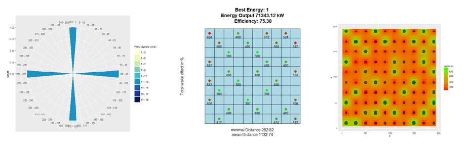
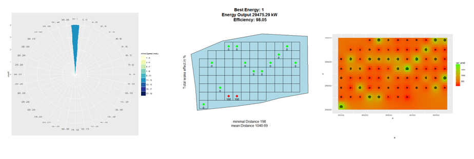
Since version 1.1, hexagonal grid cells are possible, with their center points being possible locations for wind turbines. Furthermore, rasters can be included, which contain information on the Weibull parameters (shape k, scale a). Country GeoTIFFs from the Global Wind Atlas (~250 m) are a good source; see gwa_download_country() in experimental/climate_helpers.R.

Create an input Polygon

• Input Polygon by source

library(sf)
dsn <- "Path to the Shapefile"
layer <- "Name of the Shapefile"
area <- sf::st_read(dsn = dsn, layer = layer)
plot(area, col = "blue")

• Or create a random Polygon

library(sf)
area <- sf::st_as_sf(sf::st_sfc(
  sf::st_polygon(list(cbind(
    c(0, 0, 2000, 2000, 0),
    c(0, 2000, 2000, 0, 0)))),
  crs = 3035
))
plot(area, col = "blue", axes = TRUE)

• Or draw a site on a map (GitHub clone; needs leaflet, mapedit >= 0.8, leafpm)

source("experimental/draw_shape.R")
area <- draw_shape()   # draw a polygon, then close the viewer
plot(area, axes = TRUE)

Create random Wind data

• Exemplary input Wind data with uniform wind speed and single wind direction

wind_df <- data.frame(ws = c(12, 12), wd = c(0, 0), probab = c(25, 25))
windrosePlot <- plot_windrose(data = wind_df, spd = wind_df$ws,
                              dir = wind_df$wd, dirres=10, spdmax = 20)

• Exemplary input Wind data with random wind speeds and random wind directions

wind_df <- data.frame(ws = sample(1:25, 10), wd = sample(1:260, 10))
windrosePlot <- plot_windrose(data = wind_df, spd = wind_df$ws,
                              dir = wind_df$wd)

Grid Spacing

Rectangular Grid Cells

Verify that the grid spacing is appropriate. Adapt the following input variables if necessary:

• rotor: The rotor radius in meters.
• fcr: The grid spacing factor, which should at least be 2, so that a single grid covers at least the whole rotor diameter.
• prop: The proportionality factor used for grid calculation. It determines the minimum percentage that a grid cell must cover of the area.

Make sure that the Polygon is projected in meters.

Rotor <- 20
fcr <- 9
Grid <- grid_area(area, size = (Rotor * fcr), prop = 1, plot_grid = TRUE)
str(Grid)

Hexagonal Grid Cells

Rotor <- 20
fcr <- 9
HexGrid <- hexa_area(area, size = (Rotor * fcr), plot_grid = TRUE)
str(HexGrid)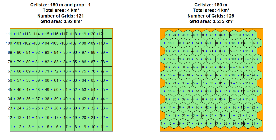

Terrain Effect Model

If terrain is TRUE in genetic_algorithm, terrain effects are taken into account. A digital elevation model and a CORINE Land Cover raster are downloaded automatically. Prefer terrain = dem (a SpatRaster) to skip the download. Per-cell height, wind multiplier, z_0, k and air density are computed once; plot_result / random_search reuse the stored terrainModel instead of downloading again. (Download a CLC raster).

To use your own land cover raster, provide its path via ccl. Surface roughness values are taken from extdata/clc_legend.csv. To use custom values, add a numeric Rauhigkeit_z column for all land cover classes, save the file with ; as delimiter, and provide its path via ccl_roughness.

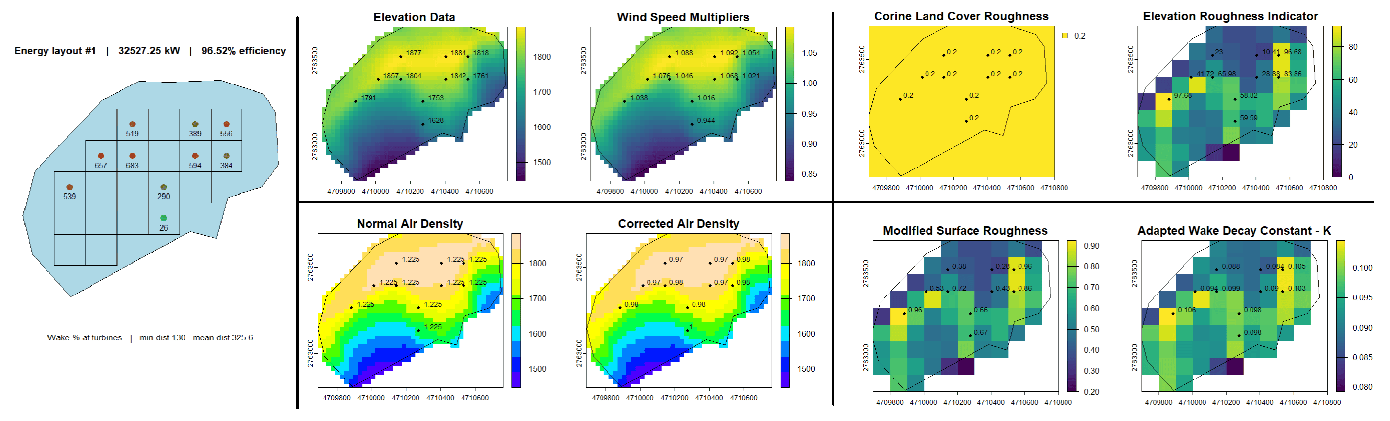
plot_result(..., terrain = TRUE) shows the full chain:

• Elevation → wind-speed multiplier (DEM / mean DEM)
• Elevation → air density (barometric; labels vs 1.225 kg/m³)
• CORINE Land Cover → land-cover roughness z_0
• Elevation roughness (terra::terrain) × CLC z_0 → modified z_0
• Modified z_0 + hub height → wake decay k = 0.5 / (h/z_0)

The modified z_0 also scales hub-height wind via the log profile (not a separate plot_result panel).

Realistic workflow (site, turbine, wind)

Clone the GitHub repo so experimental/ is available (it is not in the CRAN tarball). Browse open reference turbines at the NREL Turbine Archive.

ERA5 / Copernicus (env COPERNICUS_CLIMATE_DATA) is useful as a directional rose over time (get_era5_wind() → wind_from_era5()), but the grid is too coarse (~31 km) as a spatial wind field for siting. For mean speed per cell use Global Wind Atlas Weibull rasters (weibull = TRUE, weibull_src = list(k, a)). Hub-height correction uses reference_height (100 m for the ERA5 100 m u/v download) and rotor_height from the turbine. A met mast goes through wind_from_breeze() or wind_from_series().

library(windfarmGA)
library(sf)

source("experimental/draw_shape.R")
source("experimental/climate_helpers.R")
source("experimental/download_ERA5_historic.R")

## 1. Site: draw a polygon (or st_read a shapefile)
area <- draw_shape()
plot(area, axes = TRUE)

## 2. Turbine: IEA 3.4 MW, 130 m rotor, 110 m hub
nrel_curve_catalog()
curve <- nrel_fetch_curve("IEA_3.4MW_130")
plot_power_curve(curve)
ga_options(power_curve = curve)
rotor <- attr(curve, "rotor")           # radius in metres
hub <- attr(curve, "rotor_height")

## 3. Wind rose from ERA5 100 m u/v at the site (needs CDS key)
era5 <- get_era5_wind(area, "2021-01-01", "2025-12-31")
wind <- wind_from_era5(era5)
plot_windrose(wind, spd = "ws", dir = "wd")

##    Met mast instead of ERA5 (bReeze, or two numeric vectors):
##    library(bReeze)
##    data(winddata)
##    s40 <- set(height = 40, v.avg = winddata[, 2], dir.avg = winddata[, 14])
##    mast <- mast(timestamp(winddata[, 1]), s40)   # bReeze::mast
##    wind <- wind_from_breeze(mast)
##    wind <- wind_from_series(ws, wd)              # raw speed / direction

##    Spatial mean speed (GWA ~250 m); wind$ws is then ignored
gwa <- gwa_download_country("AUT", height = 100)  # ISO3 of the site country

## 4. Optimize
result <- genetic_algorithm(
  area = area,
  wind = wind,
  n = 12,
  rotor = rotor,
  rotor_height = hub,
  reference_height = 100,
  weibull = TRUE,
  weibull_src = gwa$weibull_src,
  terrain = TRUE,                   # DEM + CLC; needs elevatr
  fcr = 5,
  iteration = 40,
  plot = FALSE
)

## 5. Plot
print(result)
plot(result, area)
plot_result(result, area, terrain = TRUE)
plot_parkfitness(result)
plot_leaflet(result, area, which = 1)
explore_result(result, area)

source("experimental/rayshader.R")
plot_farm_3d_from_result(result, area, buffer = 5000, turbine_obj = "./experimental/wind_turbine_v1.obj")
source("experimental/plot_mapgl.R")
plot_mapgl_from_result(result, area, buffer = 8000, basemap = "satellite")


## 6. Optional: jitter turbines inside their cells (same physics as the GA)
##    Terrain is reused from result$terrainModel. Weibull rasters are not
##    stored — pass weibull_src again (that is enough, no weibull = TRUE).
refined <- random_search(
  result, area, runs = 20, best = 1, plot = FALSE,
  weibull_src = gwa$weibull_src
)
plot_random_search(refined, result, area, best = 1)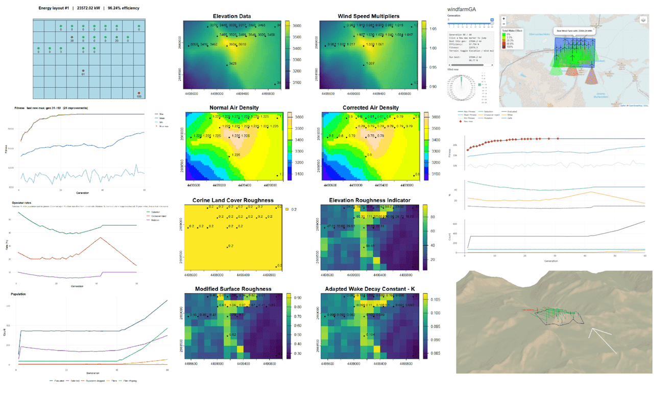

The screenshot above shows the optimized layout for a north-only wind rose. The best layout often sits in the first few upwind rows. In 2D, the arrangement looks cramped; however, wakes are in 3D. A turbine on lower ground can sit below the hub-height wake cone of a turbine further uphill and therefore is not counted as shadowed. These front rows are also at higher elevation, so the wind multiplier remains high while air density decreases less. The Leaflet map and the rayshader view (bottom right) show the same run in 2D and on the DEM.

Start an Optimization

An optimization can be initiated with the function genetic_algorithm. Search knobs that are not function arguments are session options (options(windfarmGA.*)); see Options.

• without terrain effects

result <- genetic_algorithm(
  area = area, n = 12, rotor = 20, fcr = 9, iteration = 10,
  wind = wind_df, rotor_height = 100
)

• with terrain effects

ccl <- "Source of the CCL raster (TIF)"
ccl_roughness <- "Source of the Adapted CCL legend (CSV)"

result <- genetic_algorithm(
  area = area, n = 12, rotor = 20, fcr = 9, iteration = 10,
  wind = wind_df, rotor_height = 100, terrain = TRUE,
  ccl = ccl, ccl_roughness = ccl_roughness
)

## Spatial mean speed from Global Wind Atlas (shape k, scale A).
## wind$ws is then ignored; wind$wd / wind$probab still weight directions.
source("experimental/climate_helpers.R")
gwa <- gwa_download_country("AUT", height = 100)
result_weibull <- genetic_algorithm(
  area = area, grid_method = "h", n = 12,
  fcr = 5, iteration = 10, wind = wind_df, rotor = 30,
  rotor_height = 100, weibull = TRUE, weibull_src = gwa$weibull_src
)
plot_windfarmGA(result = result_weibull, area = area)

Options

There are two layers. Arguments of genetic_algorithm() describe the site, the turbines and which GA pieces to use. Session options options(windfarmGA.*) control physics constants and the memetic search (inject, immigrants, seasons, neighbour local search). Set them before the run; they apply for the whole R session until you change them again.

ga_options()
ga_options(immigrants = 3, local_search_elites = 5, local_search_tries = 6)

The north-wind benchmark and why these search defaults exist are in inst/reports/memetic-layout-ga.md.

Arguments of genetic_algorithm()

Required: area, wind, n, rotor, rotor_height.

Site and turbines

Terrain and Weibull

GA loop

The loop is selection → set-crossover → swap-mutation → fitness.

Session options (options(windfarmGA.*))

Set with options(windfarmGA.foo = …). Defaults are assigned in .onLoad.

Physics (wake and power)

Fitness is E (/100)^w. These options change how E and are computed.

Population caps

Crossover, mutation, immigrants

On the north-wind test, extra immigrants helped the coarse search but lost to stronger neighbour local search for the last percent.

Elitism and neighbour local search

This is the memetic step. A random swap across the grid rarely fixes “one row too far inland”; a neighbour slide often does.

Adaptive rates (explore / refine / pulse)

Same three operators; only the rates change. Explore raises inject and mutation while the record is stalling (VAR selection starts near 55 %). Refine damps them toward inject 0.15, mutation 2/n, selection ~45 %. Pulse briefly raises them again so refine does not freeze.

Other

Plotting

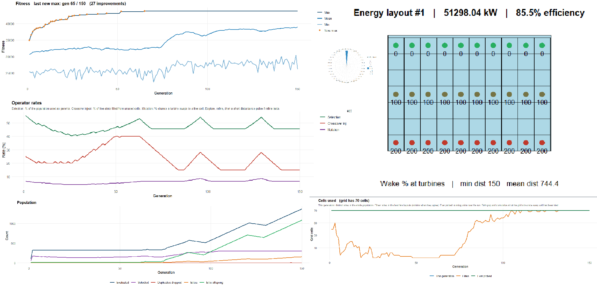
A result from genetic_algorithm() has class windfarmGA: print(result) summarises the run, plot(result, area) is plot_windfarmGA(), and explore_result(result, area) opens a one-page Shiny viewer with a Leaflet map of the best layout and a plotly figure (fitness, rates, population; click a New max marker to jump to that generation). (Suggests: shiny, leaflet, plotly).

plot_windfarmGA() pages through the best layout, fitness and operator rates, the population census, and the cell heatmap. In an interactive session each page waits for Enter. Plotly hover is used only with ask = FALSE when the plotly package is installed.

print(result)
plot(result, area)
explore_result(result, area)
plot_windfarmGA(result, area)

plot_result(result, area)                                  # best layout
plot_parkfitness(result)                                   # fitness + operator rates
plot_population(result)                                    # individuals, elites, cells
plot_generation(result, area)                              # last generation (omit generation, or pass an index)
plot_cell_heatmap(result, area)                            # which cells were tried
plot_leaflet(result, area, which = 1)                      # best on a map
plot_leaflet(result, area, orderitems = FALSE, which = 1)  # last generation
plot_evolution(result)                                     # energy + efficiency
plot_development(result)                                   # when the max improved

Package data resulthex / resultrect and sp_polygon work the same way (plot_leaflet(resulthex, sp_polygon, which = 1)).

A full documentation of the genetic algorithm is given in my master thesis.

NOTE: The implementation has changed substantially since then. Many functions and arguments have been renamed or optimized, and the internal structure of the algorithm has been reworked. As a result, the current version differs significantly from the implementation described in the thesis and calculates and converges considerably faster.

Shiny Windfarm Optimization

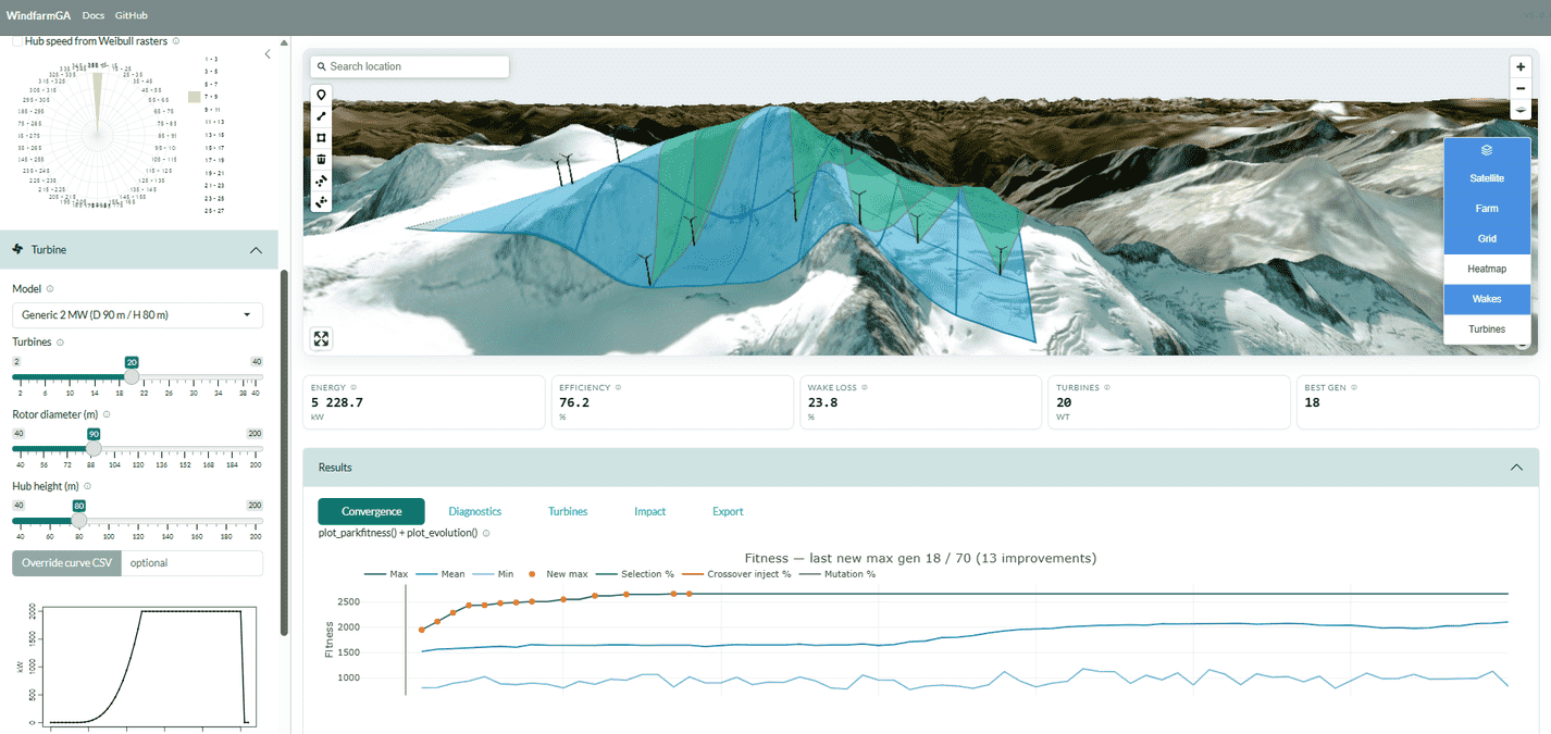
I also made a Shiny App for the Genetic Algorithm. Unfortunately, as an optimization takes quite some time and the app is currently hosted by shinyapps.io under a public license, there is only 1 R-worker at hand. So only 1 optimization can be run at a time.

These binaries (installable software) and packages are in development.
They may not be fully stable and should be used with caution. We make no claims about them.