The hardware and bandwidth for this mirror is donated by METANET, the Webhosting and Full Service-Cloud Provider.
If you wish to report a bug, or if you are interested in having us mirror your free-software or open-source project, please feel free to contact us at mirror[@]metanet.ch.

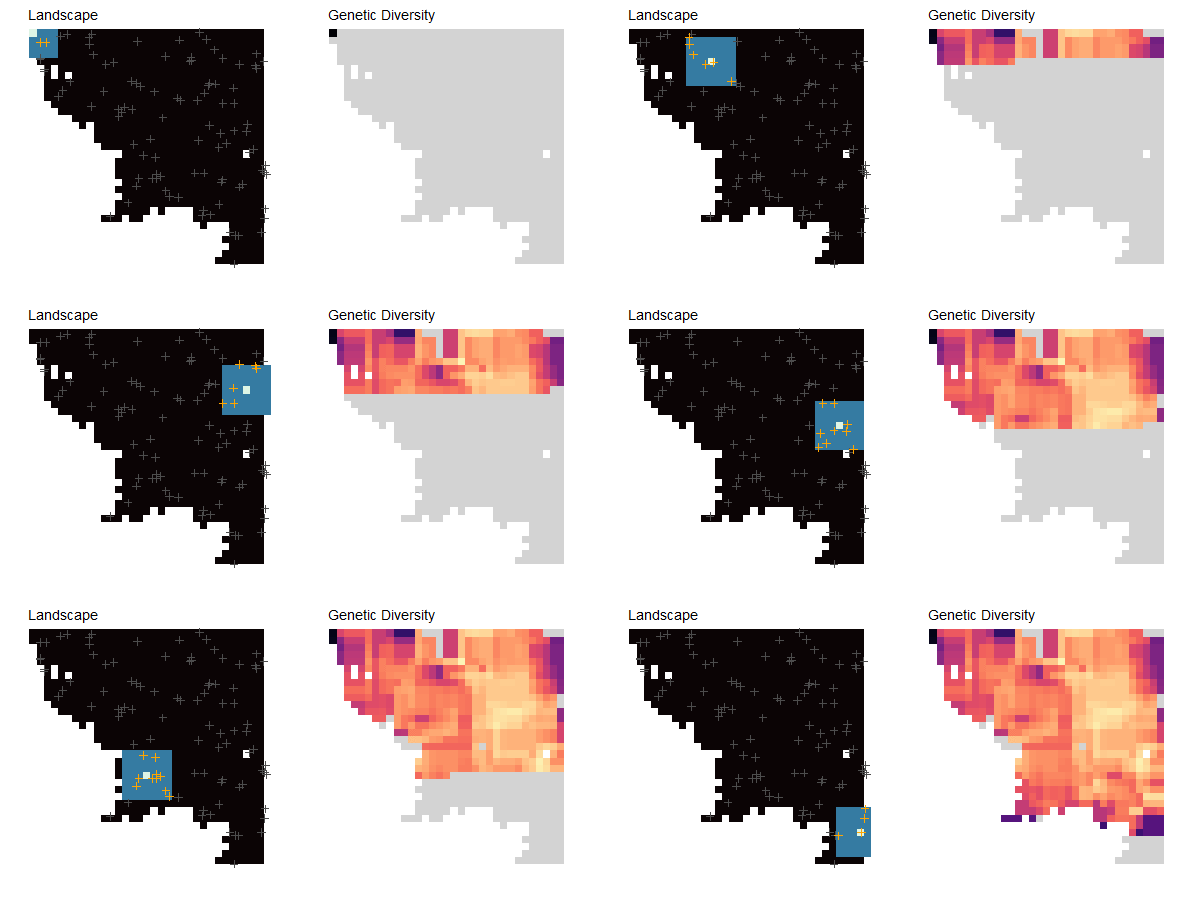
Generate continuous maps of genetic diversity using moving windows with options for rarefaction, interpolation, and masking.

Please cite the original Bishop et al. (2023) paper if you use this package:
Bishop, A. P., Chambers, E. A., & Wang, I. J. (2023). Generating continuous maps of genetic diversity using moving windows. Methods in Ecology and Evolution, 14, 1175–1181. http://doi.org/10.1111/2041-210X.14090
Checkout our Methods blog post about wingen for a quick overview of the package and its uses.
Install the released version of wingen from CRAN:
install.packages("wingen")Or install the development version from GitHub:
# install.packages("devtools")
devtools::install_github("AnushaPB/wingen")The following example demonstrates the basic functionality of wingen using a small subset (100 variant loci x 100 samples) of the simulated data from Bishop et al. (2023).
library(wingen)

# Load ggplot for plotting
library(ggplot2)

# Load example data
load_middle_earth_ex()
The core function of this package is window_gd(), which
takes as inputs a vcfR object (or a path to a .vcf file), sample
coordinates (as a data.frame, matrix, or sf object), and a raster layer
(as a SpatRaster or RasterLayer) which the moving window will slide
across. Users can control the genetic diversity statistic that is
calculated (stat), the window dimensions
(wdim), the aggregation factor to use on the raster
(fact), whether to perform rarefaction
(rarify), and other aspects of the moving window
calculations. Additional arguments for this function are described in
the vignette and function documentation.
# Run moving window calculations of pi with rarefaction
wgd <- window_gd(lotr_vcf,
  lotr_coords,
  lotr_lyr,
  stat = "pi",
  wdim = 7,
  fact = 3,
  rarify = TRUE
)

# Use ggplot_gd() to plot the genetic diversity layer and ggplot_count() to plot the sample counts layer
ggplot_gd(wgd) +
  ggtitle("Moving window pi")
ggplot_count(wgd) +
  ggtitle("Moving window sample counts")
Next, the output from window_gd() can be interpolated
using kriging with the wkrig_gd() function.
# Interpolate to a higher resolution
krige_layer <- disagg(wgd, 2)
kgd <- wkrig_gd(wgd, krige_layer)
Finally, the output from wkrig_gd() (or
window_gd()) can be masked to exclude areas that fall
outside of the study area or that were undersampled.
# Mask results that fall outside of the "range"
mgd <- mask_gd(kgd, lotr_range)
# Plot results
ggplot_gd(kgd) +
ggtitle("Kriged pi")
ggplot_gd(mgd) +
  ggtitle("Masked pi")
For an extended walk through, see the package vignette:
vignette("wingen-vignette")A pdf of the vignette can also be found here
Example analyses from Bishop et al. (2023) can be found in the paperex directory.
These binaries (installable software) and packages are in development.
They may not be fully stable and should be used with caution. We make no claims about them.