The hardware and bandwidth for this mirror is donated by METANET, the Webhosting and Full Service-Cloud Provider.
If you wish to report a bug, or if you are interested in having us mirror your free-software or open-source project, please feel free to contact us at mirror[@]metanet.ch.
Statistical theory incorrectly states that the Wilcoxon-Mann-Whitney (WMW) test examines \(\mathrm{H_0\colon F = G}\). We demonstrate this theoretical claim is untenable: the WMW statistic, when standardized, is the empirical AUC (eAUC), which measures \(P(X < Y)\) and cannot detect distributional equality. Through Monte Carlo analysis of zero-mean heteroscedastic Gaussians and corresponding asymptotic theory, we show that WMW tests \(\mathrm{H_0\colon AUC = 0.5}\) (no systematic discrimination) rather than distributional equality. Moreover, the traditional alternative hypothesis of stochastic dominance is unnecessarily restrictive; WMW is consistent against the broader alternative \(\mathrm{H_1\colon AUC \neq 0.5}\), as established by Van Dantzig (1951). We provide theoretical framework and implementation consistent with what the WMW eAUC statistic actually computes, including tie-corrected asymptotics and finite-sample bias corrections. For detalis, see (Grendár 2025).
The primary goal of wmwAUC is to provide inferences for the Wilcoxon-Mann-Whitney test of \(\mathrm{H_0\colon AUC = 0.5}\). Besides the asymtotic inferences the library provides two variants of finite-sample bias correction:
Exact Unbiased (EU) Method: Universal approach handling data with arbitrary tie patterns through the mid-rank kernel and exact finite-sample unbiased variance estimation from Hoeffding decomposition theory. Reduces correctly to the continuous case when no ties are present.
Bias-Corrected (BC) Method: Alternative for continuous data without ties, using individual component bias correction with \(O(n^{-1})\) finite-sample corrections and Welch-Satterthwaite degrees of freedom. Assumes continuous distributions with no ties.
The EU method serves as the default implementation, providing:
Universal applicability (handles any data type - continuous, discrete, or mixed)
Exact finite-sample unbiasedness (not asymptotic approximation)
Theoretically principled tie handling through mid-rank kernel
The BC method is available for users specifically working with continuous data or requiring compatibility with traditional variance estimation approaches.
Key functions include:
wmw_test(): Main testing function using EU
methodology with option to use BC method for continuous-only
data
wmw_pvalue(): WMW AUC p-values for continuous data,
based on the BC method
wmw_pvalue_ties(): WMW AUC p-values for any type of
data, based on the EU method
pseudomedian_ci(): Confidence intervals for
Hodges-Lehmann pseudomedian
quadruplot(): Diagnostics for location shift
assumption
You can install the development version of wmwAUC using
devtools::install_github('grendar/wmwAUC')Consider the setting of two zero-mean different-scale gaussians. Then the traditional \(\mathrm{H_0\colon F = G}\) of WMW test is false and \(\mathrm{H_0\colon F \neq G}\) holds.
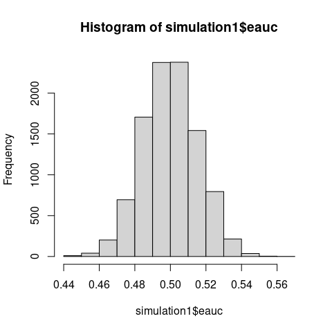
The Monte Carlo simulation demonstrates that the normalized test statistic \(U/(n_1n_2)\) which is just eAUC, concentrates asymptotically on 0.5 - the value expected under a true null hypothesis.
If WMW tested distributional equality, the test statistic should not concentrate on its null value when distributions clearly differ.
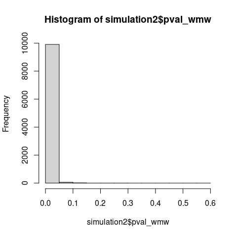
Also note that under \(\mathrm{H_0\colon F \neq G}\), p-values should concentrate near zero, yet the observed distribution is nearly uniform with a slightly elevated first bins, consistent with testing a true null hypothesis (\(\mathrm{H_0\colon AUC = 0.5}\)) using miscalibrated variance estimation.
#############################################################################
#
# Simulation 1: H0: F=G is erroneously too broad
#
#############################################################################
#
# This simulation takes several minutes to complete
# N = 10000
# n = 1000
# set.seed(123L)
# pval_wt = pval_wmw = eauc = numeric(N)
# for (i in 1:N) {
#
#   x = rnorm(n, sd = 0.1)
#   y = rnorm(n, sd = 3)
#   # wilcox.test() of H0: F = G
#   wt = wilcox.test(x, y)
#   pval_wt[i] = wt$p.value
#   # wmw_test() of H0: AUC = 0.5
#   pval_wmw[i] = wmw_pvalue(x, y)
#   # eAUC
#   eauc[i] = wt$statistic/(n*n)
#   #
# }
data(simulation1)  # List eauc, pval_wt, pval_wmw
#
Empirical AUC centered at 0.5 despite \(\mathrm{F \neq G}\).
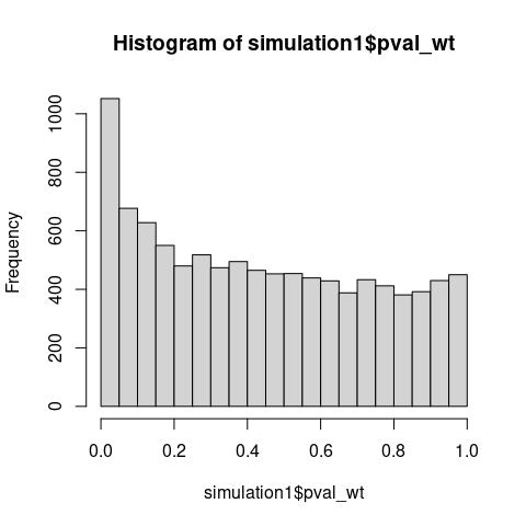
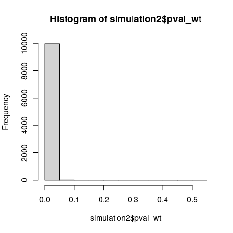
Traditional p-values under \(\mathrm{H_1}\) should concentrate near 0.
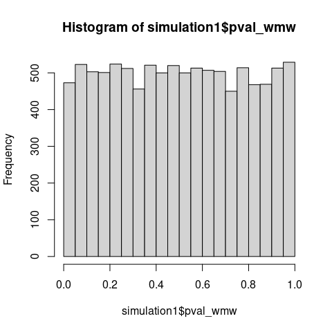
Correct p-values for testing \(\mathrm{H_0\colon AUC = 0.5}\).
The two zero-mean different-scale gaussians setting does not satisfy the traditional \(\mathrm{H_1}\) of the stochastic dominance. But, as proved by Van Dantzig in 1951, WMW is consistent for broader \(\mathrm{H_1\colon AUC \neq 0.5}\).
#############################################################################
#
# Simulation 2: H1: F stoch. dominates G is too narrow
#               WMW is consistent for broader H1: AUC != 0.5
#
#############################################################################
#
#
# This simulation takes several minutes to complete
# N = 10000
# n = 1000
# set.seed(123L)
# pval_wt = pval_wmw = eauc = numeric(N)
# for (i in 1:N) {
# #
#   # gaussians with different location and scale
#   # does not satisfy stochastic dominance
#   x = rnorm(n, 0, sd = 0.1)
#   y = rnorm(n, 0.5, sd = 3)
#   # wilcox.test H0: F = G vs H1: (F stochastically dominates G) OR (G stochastically dominates F)
#   wt = wilcox.test(x, y)
#   pval_wt[i] = wt$p.value
#   # wmw_test H0: AUC = 0.5 vs H1: AUC neq 0.5
#   pval_wmw[i] = wmw_pvalue(x, y)
#   # eAUC
#   eauc[i] = wt$statistic/(n*n)
# #
# }
data(simulation2)  # List of eauc, pval_wt, pval_wmw
# WMW detects broader alternatives than traditional stochastic dominance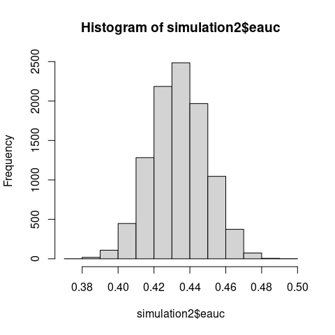
Confidence interval for the pseudomedian is obtained by inverting the
test; see pseudomedian_ci() for implementation that handles
the edge cases in the same way as wilcox.test().
In this simulation study, N = 500 MC replicates are created, of 300
samples from the standard normal distribution and 300 samples from the
Laplace distribution with location = 0, scale = 1. Properties of 95%
confidence intervals obtained under H0: AUC = 0.5 are compared with
those returned by wilcox.test().
# #############################################################################
# #
# # Simulation 3: confidence interval for pseudomedian derived under H0: AUC = 0.5
# #               MC study of N = 500 replicas
# #               x ~ rnorm(300, 0,1)
# #               y ~ rlaplace(300, 0,1)
# #
# #############################################################################
#
#
#
# This simulation takes long time to complete
# N <- 500
# n_test <- 300
#
# set.seed(123L)
# wmw_ci = wt_ci = list(N)
# eauc = pseudomed = numeric(N)
# for (i in 1:N) {
#  #
#  x_test <- rnorm(n_test, 0, 1)
#  y_test <- VGAM::rlaplace(n_test, 0, 1)
#
#  wmw_test <- pseudomedian_ci(x_test, y_test, conf.level = 0.9, pvalue_method = 'BC')
#  wmw_ci[[i]] = wmw_test$conf.int
#  wt_test <- wilcox.test(x_test, y_test, conf.int = TRUE)
#  wt_ci[[i]] = wt_test$conf.int
#  eauc[i] = wt_test$statistic/(n_test*n_test)
#  pseudomed[i] = as.numeric(wt_test$estimate)
#  #
# }
#
#
data(simulation3)  # List of wmw_ci, wt_ci, eauc, pseudomedian
#
# Average across MC of confidence intervals obtained under H0: AUC=0.5
colMeans(simulation3$wmw_ci)
#> [1] -0.1701256  0.1735400
# Average across MC of confidence intervals from wilcox.test()
colMeans(simulation3$wt_ci)
#> [1] -0.1754612  0.1790767
#
# Average across MC of eAUC
mean(simulation3$eauc)
#> [1] 0.5004063

# Coverage
length(which((simulation3$wmw_ci[,1] < 0) & (simulation3$wmw_ci[,2] > 0)))
#> [1] 470
length(which((simulation3$wt_ci[,1] < 0) & (simulation3$wt_ci[,2] > 0)))
#> [1] 473

# Mean pseudomedian
mean(simulation3$pseudomed)
#> [1] 0.001776475Real data analyzed by WMW test of no group discrimination.
data(gemR::MS)
da <- MS

# preparing data frame
class(da$proteins) <- setdiff(class(da$proteins), "AsIs")
df <- as.data.frame(da$proteins)
df$MS <- da$MSwmd <- wmw_test(P19099 ~ MS, data = df, ref_level = 'no')
wmd
#>
#> Wilcoxon-Mann-Whitney Test of No Group Discrimination
#>
#> data: P19099 by MS (n1 = 37, n2 = 64)
#> groups: yes vs no (reference)
#> U = 1726, eAUC = 0.729, p-value = 0.000007, method = EU
#> alternative hypothesis for AUC: two.sided
#> 95 percent confidence interval for AUC (hanley):
#> 0.623 0.835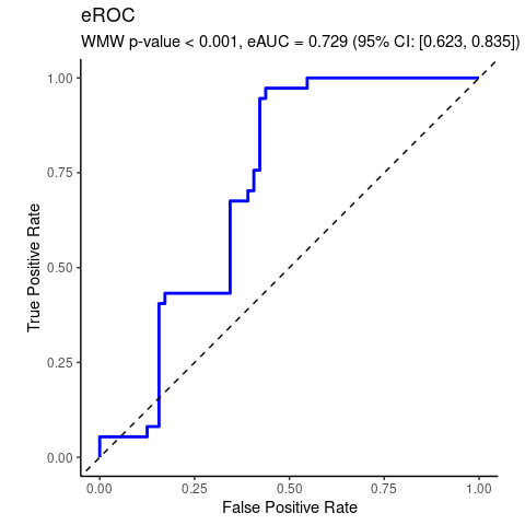
Synthetic data illustrating the special case of location shift assumption.
data(Ex2)
da <- Ex2

# WMW test
wmd <- wmw_test(y ~ group, data = da, ref_level = 'control')
wmd
#>
#>         Wilcoxon-Mann-Whitney Test of No Group Discrimination
#>
#> data: y by group (n1 = 100, n2 = 100)
#> groups: case vs control (reference)
#> U = 3705, eAUC = 0.370, p-value = 0.001106, method = EU
#> alternative hypothesis for AUC: two.sided
#> 95 percent confidence interval for AUC (hanley):
#>  0.294 0.447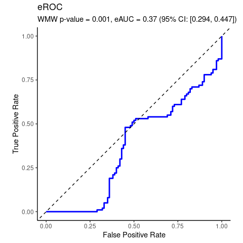
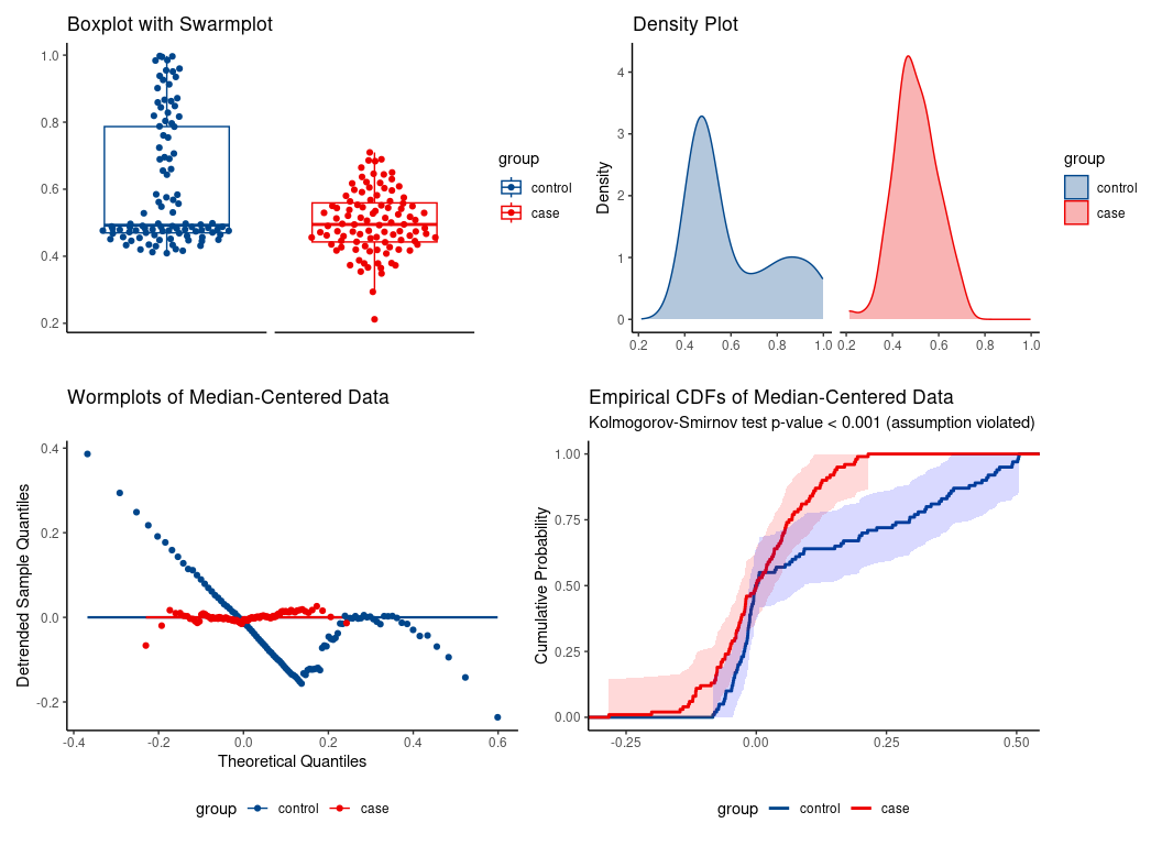 location-shift assumption not tenable.
Erroneous use of location-shift special case of WMW would falsely conclude significant median difference despite identical medians.
#>
#>         Wilcoxon-Mann-Whitney Test of No Group Discrimination
#>
#> data: y by group (n1 = 100, n2 = 100)
#> groups: case vs control (reference)
#> U = 3705, eAUC = 0.370, p-value = 0.001106, method = EU
#> alternative hypothesis for AUC: two.sided
#> 95 percent confidence interval for AUC (hanley):
#>  0.294 0.447
#>
#> Location-shift analysis (under F1(x) = F2(x - delta)):
#> alternative hypothesis for location: two.sided
#> Hodges-Lehmann median of all pairwise distances:
#>  -0.048 [location effect size: eAUC = 0.370]
#> 95 percent confidence interval for median of all pairwise distances:
#>  -0.084 -0.037
Indeed, the medians are essentially the same:
median(da$y[da$group == 'case'])
#> [1] 0.4949383
median(da$y[da$group == 'control'])
#> [1] 0.4926145WMW applied to another real-life data set.
data(wesdr)
da = wesdr
da$ret = as.factor(da$ret)
# WMW
wmd <- wmw_test(bmi ~ ret, data = da, ref_level = '0')
wmd
#>
#>         Wilcoxon-Mann-Whitney Test of No Group Discrimination
#>
#> data: bmi by ret (n1 = 278, n2 = 391)
#> groups: 1 vs 0 (reference)
#> U = 59417.5, eAUC = 0.547, p-value = 0.035168, method = EU
#> alternative hypothesis for AUC: two.sided
#> 95 percent confidence interval for AUC (hanley):
#>  0.502 0.591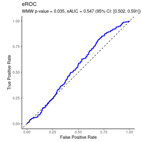
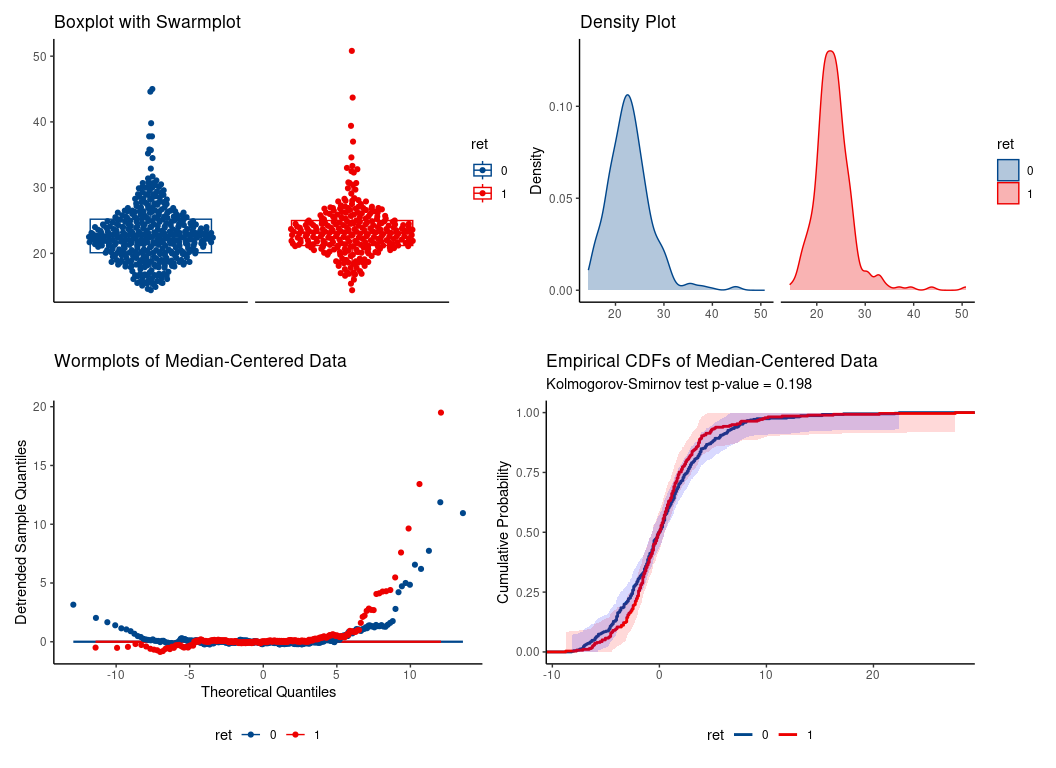 hence, location shift assumption is tenable.
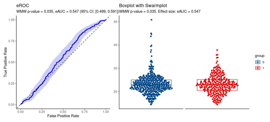
wml <- wmw_test(bmi ~ ret, data = da, ref_level = '0',
                 ci_method = 'boot', special_case = TRUE, n_grid = 100)
wml
#>
#>         Wilcoxon-Mann-Whitney Test of No Group Discrimination
#>
#> data: bmi by ret (n1 = 278, n2 = 391)
#> groups: 1 vs 0 (reference)
#> U = 59417.5, eAUC = 0.547, p-value = 0.035168, method = EU
#> alternative hypothesis for AUC: two.sided
#> 95 percent confidence interval for AUC (boot):
#>  0.499 0.591
#>
#> Location-shift analysis (under F1(x) = F2(x - delta)):
#> alternative hypothesis for location: two.sided
#> Hodges-Lehmann median of all pairwise distances:
#>  0.600 [location effect size: eAUC = 0.547]
#> 95 percent confidence interval for median of all pairwise distances:
#>  0.294 0.906
Plot
AI-assisted code generation via Claude Pro by Anthropic was used in development. All generated content was verified, tested, and enhanced by the package author.
These binaries (installable software) and packages are in development.
They may not be fully stable and should be used with caution. We make no claims about them.