
The hardware and bandwidth for this mirror is donated by METANET, the Webhosting and Full Service-Cloud Provider.
If you wish to report a bug, or if you are interested in having us mirror your free-software or open-source project, please feel free to contact us at mirror[@]metanet.ch.

This package adds some extra functionality and plots to the xpose
framework. This includes some plots that have been missing in
translation from xpose4,
but also some useful features that truly extend the capabilities of what
can be done with xpose.
There are a few bugfixes here and functionality which could easily be
suggested as pull requests to the parent package. Given the size and
broad use of xpose, it appears even minor pull requests
take some time to implement. As such, this package implements those
features directly and if at any point in the future these are added
(perhaps in a better state) to the parent package, they will be
deprecated if this package is in active use.
For those wondering, conflicted is used
to manage bugfix conflicts, so users should be comfortable loading
packages in any order.
The package can be installed from CRAN:
install.packages("xpose.xtras")The typical github installation will also work.
pak::pak("jprybylski/xpose.xtras")The main github branch is reserved for CRAN release-ready versions. The dev branch is usually ahead if there is active development.
pak::pkg_install("jprybylski/xpose.xtras@dev")The grandparent package, xpose4, used to have a nice
collection of figures and documentation that is referred to as a
“bestiarium”. The documentation site for this package serves as a
complete bestiary, but see the uncommented examples below as a sort of
menagerie. There is no assumption that these examples are
self-explanatory, but hopefully users familiar with xpose
will recognize the new (and renewed) tools made available by
this package.
described <- xpdb_x %>%
  set_var_labels(AGE="Age", MED1 = "Digoxin", .problem = 1) %>%
  set_var_units(AGE="yrs")  %>%
  set_var_levels(SEX=lvl_sex(), MED1 = lvl_bin())
eta_vs_contcov(described,etavar=ETA1, quiet=TRUE)
#> `geom_smooth()` using formula = 'y ~ x'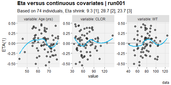
eta_vs_catcov(described,etavar=ETA1, quiet=TRUE)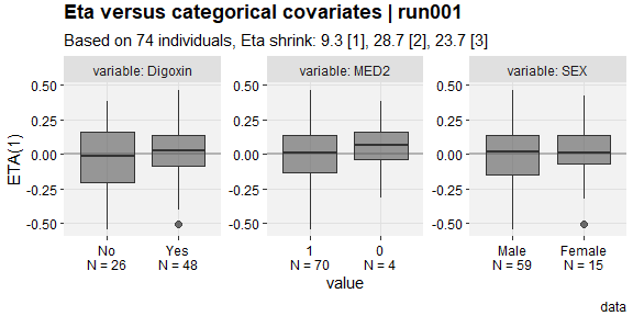
pheno_set %>%
  focus_qapply(backfill_iofv) %>%
  dofv_vs_id(run6, run9, quiet = TRUE)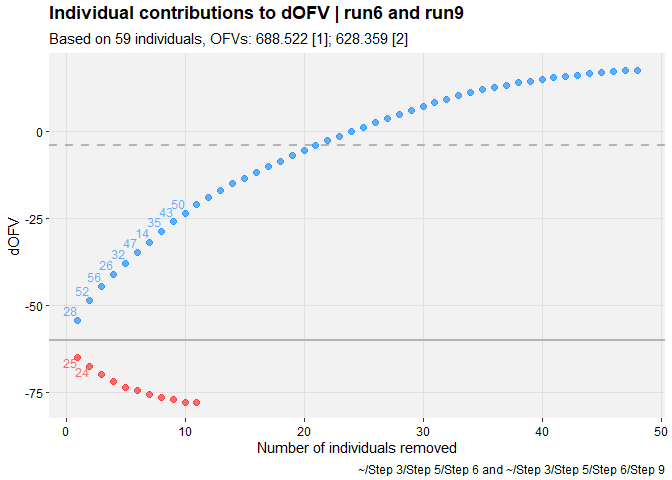
pkpd_m3 %>%
  set_var_types(catdv=BLQ,dvprobs=LIKE) %>%
  set_dv_probs(1, 1~LIKE, .dv_var = BLQ) %>%
  set_var_levels(1, BLQ = lvl_bin()) %>%
  catdv_vs_dvprobs(quiet=TRUE)
#> `geom_smooth()` using method = 'gam' and formula = 'y ~ s(x, bs = "cs")'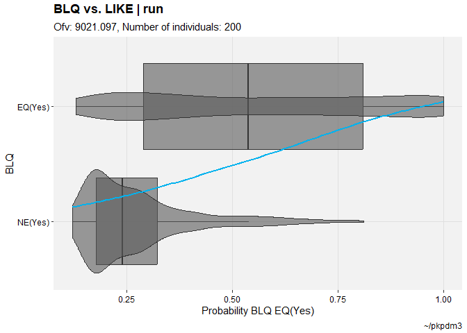
nlmixr2_m3 %>%
  set_var_types(catdv=CENS,dvprobs=BLQLIKE) %>%
  set_dv_probs(1, 1~BLQLIKE, .dv_var = CENS) %>%
  set_var_levels(1, CENS = lvl_bin()) %>%
  roc_plot(quiet = TRUE)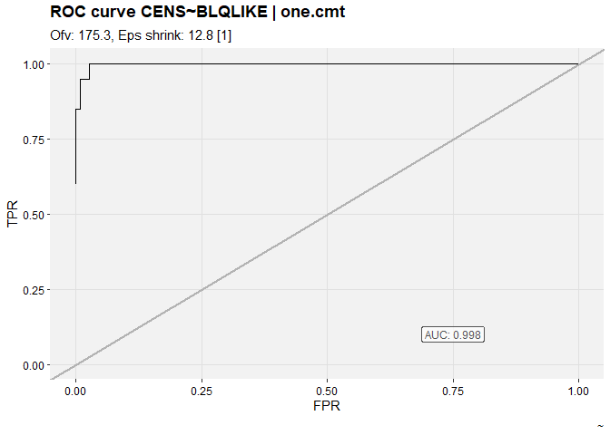
These binaries (installable software) and packages are in development.
They may not be fully stable and should be used with caution. We make no claims about them.